

1 Introduction
How much is enough? How much data do we need to have an adequate record of a language? These are key questions for language documentation. Though we concur in principle with Himmelmann’s (Reference Himmelmann1998: 166) answer, that ‘the aim of a language documentation is to provide a comprehensive record of the linguistic practices characteristic of a given speech community’, this formulation is extremely broad and difficult to quantify. Where does ‘comprehensive’ stop? The syntax? A dictionary of a specified minimum size (is 1000 words enough? 10,000?), or should we aim to describe the ‘total’ lexicon? Steven Bird posted the following enquiry to the Resource Network for Linguistic Diversity mailing list (21/11/2015):
Have any endangered language documentation projects succeeded according to this [Himmelmann’s] definition? For those that have not (yet) succeeded, would anyone want to claim that, for some particular language, we are half of the way there? Or some other fraction? What still needs to be done? Or, if a comprehensive record is unattainable in principle, is there consensus on what an adequate record looks like. How would you quantify it?
Quantifying an answer to the ‘Bird–Himmelmann problem’ is becoming more acute as funding agencies seek to make decisions on how much fieldwork to support on undocumented languages, and digital archives plan out the amount of storage needed for language holdings.
As a first step towards answering questions of this type in a quantifiable way, there are good reasons to begin with the units of language structure that are analytically smallest, the least subject to analytic disagreement, and that have the highest frequency in running text. For example, both /ð/ and /ə/ will each occur more frequently than the commonest word in English, /ðə/ ‘the’, since both occur in many other words, and more significantly, they will occur far more often than e.g. intransitive verbs, relative clauses or reciprocal pronouns. As a result, asking how much material is needed in order to sample all the phonemes of a language sets a very low bar. This bar sets an absolute minimum answer to the Bird–Himmelmann problem as it should be both relatively easy to measure because of the frequency of the elements, and obtainable with small corpus sizes. The relevant questions then become: How much text do we need to capture the full phoneme inventory of a language? What proportion of the phoneme inventory can we expect to sample in a text of a given length? Setting the bar even lower, we will define ‘capture a phoneme’ as finding at least one allophone token of a phoneme; this means that we are not asking the question of how one goes about actually carrying out a phonological analysis, which brings in a wide range of other methods and would require both more extensive and more structured data (e.g. minimal pairs sometimes draw on quite esoteric words).
To tackle the phoneme capture problem, we draw on the collection of illustrative transcribed texts (henceforth Illustrative Texts) that have been published in Journal of the International Phonetic Association as Illustrations since 1975.Footnote 1
The vast majority of these (152) are based on translations of a traditional story from Mediterranean antiquity, the ‘North Wind and the Sun’ (NWS), but a small number (eight) substitute other texts. Each of these publications presents, firstly, a phonemic statement, including allophones of the language’s phoneme inventory, and secondly a phonetic (and orthographic) transcription of the Illustrative Text together with an archive of sound recordings.
This corpus, built up over 43 years, represents a significant move to gathering cross-linguistically comparable text material for the languages of the world. This remains true even though the original purpose of publishing NWS texts in JIPA Illustrations was not to assemble a balanced cross-linguistic database of phonology in running text, and it was not originally planned as a single integrated corpus.Footnote 2 However, a number of features of the NWS text make it a useful research tool for the questions we are investigating in this paper. First, by being a semantically parallel text it holds constant (more or less) such features as genre and length. Second, JIPA’s policy of including the phonemic inventory in the same paper, together with a broad phonetic transcription (with some authors providing an additional narrow transcription), conventions for the interpretation of the transcription, and an orthographic transcription, establish authorial consistency between phonemic analysis and transcription – notwithstanding occasional deviations to be discussed below. Third, sound files are available for a large number of the languages and can be used for various purposes, such as measuring the average number of phonemes per time unit, something we will also draw on in our analysis. These characteristics make JIPA’s Illustrations a well-curated and incremental collection of great utility, numbering 160 language varieties from every continent at the time of our analysis, though with significant geographical bias towards Europe and away from Melanesia, parts of Africa, north Asia and the Amazon.
The use of the NWS text was originally attuned to English phonology, approaching the ideal of being panphonic – representing every phoneme at least once – though as we shall see it generally falls short of total phoneme sampling, even in English. The design of the NWS text as near-panphonic for English means it does not constitute a phonemically random sampling of phoneme frequencies since the need for coverage was built into the text design. But by their nature panphones, and their better-known written relatives pangrams, relinquish this role once translated into other languages. Thus, the English pangram The quick brown fox jumps over the lazy dog ceases to be pangrammic in its Spanish translation El rápido zorro salta sobre el perro perezoso, which lacks the orthographic symbols c, d, f, g, h, j, (k), m, n, ñ, q, u, v, w, x and y. And conversely the German pangram Victor jagt zwölf Boxkämpfer quer über den großen Sylter Deich, translated into English Victor chases twelve boxers diagonally over the great Sylt dyke, misses the letters f, j, m, q, u, w and z. For our purposes here, the fact that translations do not maintain panphonic status (except perhaps in very closely related varieties) is, ironically, an asset for the usefulness of the Illustrative Texts collection. This is because the further that translations move away from the source language, the closer they come to more natural samplings of phonemes in running text.
To explore the Bird-Himmelmann problem we will use the JIPA Illustrative Texts corpus to answer a range of interlinked questions.
First, how representative of a language’s phoneme inventory is the NWS transcript; that is, how much coverage of the inventory is provided by the transcript?
Second, how long does it take to recover a given phoneme, and are some phonemes less likely to appear than others? Many characteristics of language follow a Zipf-like frequency distribution such that a few tokens are observed many times, while most are observed infrequently (Zipf Reference Zipf1932, Reference Zipf1936). If phonemes follow this pattern, then a potential consequence is that there might be no Bird–Himmelmann horizon where we have fully described a language’s inventory since any new observation could find a new unobserved token. Alternatively, phonemes might follow a different frequency distribution, reflecting the fact that even the rarest of phonemes in a language need to occur at a certain frequency in order to survive as systemically organised, contrastive units, and for children to quickly learn their status as units in the phoneme system.
Third, given the rate at which we are recovering phonemes, can we predict how much text is needed to recover a language’s inventory, once we know the number of phonemes?
Fourth, are phonemes that are cross-linguistically rarer less likely to appear in the Illustrative Texts of languages which contain them – in other words, if a language contains phonemes A and B, A being cross-linguistically commoner than B, is A more likely to appear in the Illustrative Text, and in a given language will the token frequencies of cross-linguistically rarer phonemes be less than those for cross-linguistically commoner ones?
2 Language sample
A total of 158 speech varieties from 156 published Illustrations from 1975 to 2017 are included in our study. These represent virtually all published texts in the Illustrations series up to December 2017. Three Illustrations had insurmountable problems for coding purposes and were discarded: American English from Central Texas (de Camp Reference de Camp1978), American English from Eastern Massachusetts (de Camp Reference de Camp1973) and Kumzari (Anonby Reference Anonby2011). There are 137 distinct languages, with some languages (e.g. English, Dutch, Chinese) represented by multiple dialects, and one language (Dari Afghan Persian) represented by both a formal and informal register. We assigned a file to each speech variety presented in a JIPA Illustration; the file contains a mixture of identifying material, and extracted data relevant to this research. The identifying material contains the Illustration’s digital object identifier, the ISO 639-3 code, if available, and the name of the speech variety as presented in the Illustration. The names reflect the fact that the speech varieties covered in the Illustrations range in status from ‘language’ to minority ‘dialect’.
3 Data coding
The content that was extracted from each Illustration included the consonant phoneme inventory, the vowel phoneme inventory, the total number of phonemes in the language variety, the Illustration text transcription, symbols in the Illustration text transcription that were irrelevant to the phoneme inventory (e.g. intonation boundaries and punctuation) and notes. If the Illustrative text was available as an audio file we recorded the length of the audio file, except for a few audio passages that we deemed to exhibit significant disfluencies or side-passages, such as questions to the recorder, in which case we excluded this audio file from our measurements.
The phoneme inventories contained the phonemes identified by the Illustration authors, along with their allophones as recoverable from the Illustration. In some cases, the allophones were explicitly discussed in the Illustrations, in other cases allophones were assigned based on our analysis of the Illustration text transcript and author’s discussion of conventions. In most languages the transcripts also contained sounds which could not be assigned to the phoneme inventory (see below). The phonemic analyses found in the Illustrations are not necessarily the same as presented by other authors elsewhere, but for this study, the source material on each language was based exclusively on the information presented in the JIPA Illustrations, so as to ensure internal consistency between analysis and corpus.
Some of the issues encountered in the preparation of the data included the representation of allophones, narrow phonetic versus broad phonemic transcriptions, typographical errors, and consistency across languages.
As noted above, not all allophones were discussed in the Illustrations, meaning that we often needed to make judgement calls on when to label a sound segment as an allophone. This was generally only done with evidence from the transcript, and/or supporting comments from the author in their discussion, and/or supporting evidence from comparing the orthographic version of the text with the phonetic/phonemic version of the text. This was done in a conservative manner. As non-experts in the varieties of languages in the Illustrations, we were mindful of avoiding errors in the assignment of allophones. The first time allophones were assigned was when structural and word-list data from the Illustrations were initially entered into language files. The second time allophones were assigned was following an initial parsing of the passage. At this stage, although it was possible to assign many sounds as allophones, there was a substantial residue of sounds which we designated as errors.
Examples of errors found in the initial parsing that were then subsequently included in the phonemic inventory (either as phonemes or allophones) included: (i) instances where a phoneme wasn’t entered into the phoneme chart; (ii) instances where allophones weren’t identified in the initial coding of data; and (iii) instances of phonetic processes marked in the text transcription, but not discussed in the paper. An example of the first phenomenon is that /w/ was not included in the phoneme inventory chart for Setswana (Bennett et al. Reference Bennett, Maxine, Justine, Tracey and Tsholofelo2016), but from discussion in the paper, and notably the list of phonemes with example words, it was clearly a phoneme. An example of the second phenomenon is that on first parsing of Lower Xumi (Chirkova & Chen Reference Chirkova and Yiya2013b) schwa was found in the Illustrative text, but was unaccounted for in the phoneme inventory. It was assigned as an allophone of /u/ based on a footnote concerning the prosodically unstressed directional prefix (Chirkova & Chen Reference Chirkova and Yiya2013b: 367). An example of the third phenomenon can be seen in the Illustration of Tukang Besi (Donohue Reference Donohue1994), in which the length mark occurs on both consonants and vowels, but length/gemination is not discussed in the paper. Likewise in the Illustration of Mambay (Anonby Reference Anonby2006), while contrastive length is discussed in the paper, in the text transcription some vowels are marked as extra-long (e.g. ‹óːː›), with no explanation.
In some cases, errors found in the initial parsing could not be allocated to the phoneme inventory as either phonemes or allophones. For example, in the Illustration of the dialect of Maastricht (Gussenhoven & Aarts 1999) the symbol ‹r› appears in the transcript twice, with no discussion of this sound elsewhere in the paper, while in the Illustration of Lyonnais (Francoprovençal; Kasstan Reference Kasstan2015) the symbol ‹œ› appears in the transcript with no discussion of this sound elsewhere in the paper.
Members of the International Phonetic Association agreed at the 1989 Kiel Convention that the transcriptions of the Illustrative Text ‘may be in a broad, phonemic, form, allowing the interpretation conventions to specify allophonic variations that occur; or it may in itself symbolize some of the phonetic phenomena in the recording’ (IPA 1990: 41). While this allows authors to use the transcription to different purposes, if all symbols used in a narrow transcription are not explicitly discussed in the text, it can be difficult for readers unfamiliar with the language to tease apart language-wide phonological processes and individual speakers’ idiosyncrasies. The practice, adopted by many authors, of providing both a broad transcription and a narrow transcription helps in this regard. In those Illustrations that contained a more narrow transcription, there was a significantly higher number of errors following parsing than for those Illustrations that contained a broad or phonemic transcription.
When we encountered mismatches between the inventory of phones in the Illustrative Text and those listed in the first part of the Illustration, we checked back to determine the two main categories of discrepancy. In some instances this is because the authors of Illustrations have made typographical errors (typos), while in others these occurred in the first phases of our data entry process. After initially parsing the data, errors were checked to identify which category they fell into. Several patterns emerged amongst author typos. Impressionistically, the most common typo across languages was the symbol ‹y› for the palatal approximant [j], e.g. Illustration of Assamese (Mahanta Reference Mahanta2012) and Illustration of Nen (Evans & Miller 2016). This typo is a specific example of a more general type, whereby an orthographic symbol is used instead of a phonetic symbol (in the case that the orthography is based on a Romanised script). With the orthographic versions of the Illustrative Text transcription provided in each Illustration, it is a straightforward process to establish when this kind of typo has occurred. However, it is not necessarily as straightforward for an author who is accustomed to reading and writing a language both phonetically and orthographically to keep the two systems distinct, and there appears to have been a significant amount of symbol migration in both directions. It appears very easy to mix symbols from one system into the other, and no doubt very difficult for an author to always consciously separate the two systems.
The final issue that was encountered during the data entry phase was that of consistency across language varieties. The main problem areas were the marking of length and geminates, the treatment of diphthongs, and the representation of tones.
3.1 Length/gemination
In different parts of the world there are different traditions for referring to duration phenomena for vowels and consonants. This is reflected in the Illustrations, with some authors referring to ‘length’ while others refer to ‘gemination’. Further, in one Illustration an author may use the terms interchangeably (e.g. Dawd & Hayward Reference Dawd and Hayward2002), while in another Illustration again an author may (for good reason) employ one terminology for consonants and the other for vowels. For example, in the Tamil Illustration (Keane Reference Keane2004) and the Shilluk Illustration (Remijsen, Ayoker & Mills 2001) duration phenomena for vowels are referred to as ‘length’ and duration phenomena for consonants are referred to as ‘gemination’. The representation of length and gemination also varies across the Illustrations. Two methods are used, namely to use a double letter symbol (e.g. [d]∼[dd], [e]∼[ee]), or to use the length symbol (e.g. [d]∼[dː], [e]∼[eː]). For some languages it is necessary to identify three different length types, in which case triple letter symbols may be used (e.g. [d]∼[dd]∼[ddd], [e]∼[ee]∼[eee]) or the distinction is made using an additional length symbol (e.g. [d]∼[dˑ]∼[dː], [e]∼[eˑ]∼[eː]). Across the Illustrations both of these methods are found, whether for length or for gemination. For ease of comparison in this study, no distinction has been made between length and gemination, and both are presented in the language files using length symbols. That is, in languages in which length/gemination was marked by double or triple letter symbols, the notation was changed to use the length symbols.
3.2 Diphthongs vs. vowel sequences
The Illustrations also vary in how authors analyse sequences of vowels. This possibly reflects the fact that diphthongs tend to be under-described: ‘when diphthongs come into play, the textbooks tend to remain somewhat fuzzy with respect to procedures for working out a potential diphthong inventory and for further analysis and systematization’ (Geyer Reference Geyer, Haig, Nicole, Stefan and Claudia2011: 178). In some Illustrations diphthongs are included in the phoneme inventory, while in others they are not. In some languages the set of possible diphthongs is very small, and in such languages the few diphthongs are easily listed in the phoneme inventory (e.g. American English: Southern Michigan (Hillenbrand Reference Hillenbrand2003)). In others, there is a much larger number of possible diphthongs, and in such cases authors either add all the possibilities to the phoneme inventory (e.g. Estonian (Asu & Teras 2009) and Bengali (Khan Reference Khan2010)) or leave them out altogether (e.g. Ersu (Chikova et al. 2015)). In this study we have simply followed the authors’ lead in including diphthongs in the phoneme inventory or not, as the case may be. Frequently, in the languages for which a large number of diphthongs have been identified, these diphthongs do not appear in the transcript and are therefore missing. This problem would not have surfaced had the diphthongs not been listed. To this extent our findings are hostage to the specific analyses advanced by the authors of the Illustrations.
3.3 Tonal contrasts
At the 1989 Kiel Convention two systems for the representation of tone were approved, namely diacritical tone marks and tone letters. In the report on the Convention it was noted that the two systems are ‘inter-translatable’ (IPA 1989: 77). While both these systems are indeed used in Illustrations, other systems using numbers (e.g. Itunyoso Trique (DiCanio Reference DiCanio2010)) or letter abbreviations (e.g. Lower Xumi and Upper Xumi; Chirkova & Chen Reference Chirkova and Yiya2013b, and Chirkova, Chen & Kocjančič Antolik Reference Chirkova, Chen and Kocjančič2013) are also used. In addition, cross-linguistically, tone has many functions, and there is also variation in the unit with which tone is associated (e.g. phoneme, syllable or word). The multiplicity of systems for marking tone, in addition to the myriad realisations of tone in individual languages, make its comparison using the Illustrations untenable for this study, and with considerable regret we have made the pragmatic decision not to include tonal contrasts in the phoneme inventory. As a result of this decision, the findings of our study cannot be taken to apply to tonal phonemes, a question that must await further study.
This leaves the problem of how to make sure that orthogonal dimensions of phonemic contrast (e.g. vowel quality) are examined without being tangled up in the difficulties posed by tonal representations. We dealt with this in the following way. In the data files for each of the tonal language varieties from the Illustrations tone was reproduced as it was marked in its JIPA Illustration. In the case of languages for which diacritical tone marks have been used, all possible tonal realisations of a vowel (or in some cases consonant) phoneme were represented as allophones of the vowel (or consonant) phoneme. While linguistically speaking tone is not allophonic, by representing it in this way in the data files it could be eliminated as a variable from the corpus. This is illustrated by the Shilluk case study below.
3.4 Illustration of an Illustration: Shilluk
Shilluk (Remijsen et al. 2011) is a Western Nilotic language spoken in Southern Sudan. Entering data on Shilluk we ran into some of the challenges discussed above. Here the consonant inventory, vowel inventory and transcript (which for this Illustration is phonemic) as found in our language file have been reproduced.
Consonant inventory
Vowel inventory
Transcription


Phonemes in the consonant and vowel inventories are separated by commas. The sounds in parentheses following some of the phonemes are allophones of that phoneme: e.g. p(p, b, f, w) means that /p/ is the phoneme, and [p], [b], [f] and [w] are allophonic realisations. The consonant allophones were discussed in the Illustration and added into the phoneme inventory based on the author’s discussion. Shilluk has a three-way distinction between length in vowels, which in the paper is written as single letter for short, double letter for long and triple letter for overlong (e.g. o, oo, ooo). In our data file this was changed to be consistent across languages, so that a single letter symbol represents short vowels, the half-long symbol represents long vowels and the long symbol represents overlong vowels. Consonantal gemination is discussed by the authors in the Illustration. It is considered a phonological process rather than phonemic (and is often not phonetically realised). There is only one example of it in the transcription. Because of its non-phonemic status [nː] was added as an allophone of /n/. In the paper, as with vowel length, the authors indicated geminate consonants by doubling the letter symbol. In our data we have used the length symbol.
The Illustration authors identify seven tonemes for Shilluk, which they mark on vowels using diacritics (Remijsen et al. 2011: 118). The seven tones are: Low (cv́c), Mid (cv̄c), High (cv̀c), Rise (cv̌c), Fall (cv̂c), High Fall (cv̂́c), and Late Fall (cv́c̀). Due to the difficulties discussed above in including tone in this study, tone is accounted for in the language file as an allophonic feature (e.g. iˑ(iˑ, íˑ, īˑ, ìˑ, ǐˑ, îˑ)). This means that if a vowel of a particular quality appears in the transcript, regardless of its tone, only the vowel quality is measured in the study, while the tones are excluded. Following initial parsing of Shilluk, data entry errors were found, where some of the possible vowel–tone combinations were missing from the phoneme inventory. These were rectified, resulting in the vowel phoneme inventory appearing as above. There are no instances of the late fall tone occurring in the NWS transcription. If there had been, the tone marking on the consonant would have been added into the phoneme inventory, with consonants taking tones being added in as allophones, in the same way in which this was done for vowels.
4 Overview of the JIPA Illustration text corpus
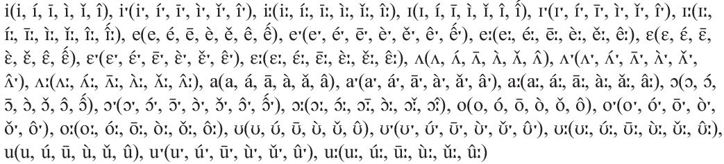
Our JIPA Illustrative Text corpus contains 158 varieties from 137 languages (Figure 1). The phoneme inventories range from 18 (Amarasi; Edwards Reference Edwards2016) to 97 (Estonian; Asu & Teras 2009), with a median of 39.5 phonemes (s.d. = 14.7 phonemes). The median length of the Illustrative Text transcript is 591 segment tokens (s.d. = 181.0 tokens), with the shortest transcript belonging to Spokane (n = 262; Carlson & Esling Reference Carlson and Esling2000) and the longest to Shipibo (n = 1690, Valenzuela; Piñedo & Maddieson Reference Valenzuela, Piñedo and Maddieson2001).

Figure 1 Histograms showing distributions of the number of phonemes, for each language: (a) the size of the phoneme inventory; (b) the length of the Illustration transcript; (c) the number of phonemes not found in the transcript; and (d) the number of unexpected phonemes in the transcript (errors).
The sample of languages is global (Figure 2) but heavily biased towards Indo-European languages (n = 66, 41.7 %), and to a lesser degree Austronesian (n = 16, 10.1%) and Atlantic-Congo (n = 13, 8.2%), Sino-Tibetan (n = 11, 7.0%) and Afro-Asiatic (n = 9, 5.7%). Language families that are noticeably under-sampled are those from the Americas (e.g. Oto-Manguean, Arawakan, Uto-Aztecan, Mayan), Australia (e.g. Pama-Nyungan, Gunwinyguan), Asia (e.g. Dravidian, Austro-Asiatic, Hmong-Mien, Tai-Kadai) and New Guinea (e.g. Trans-New Guinea, Torricelli, Sepik). These biases simply reproduce the sampling bias in the JIPA Illustrations, and in linguistics more generally.
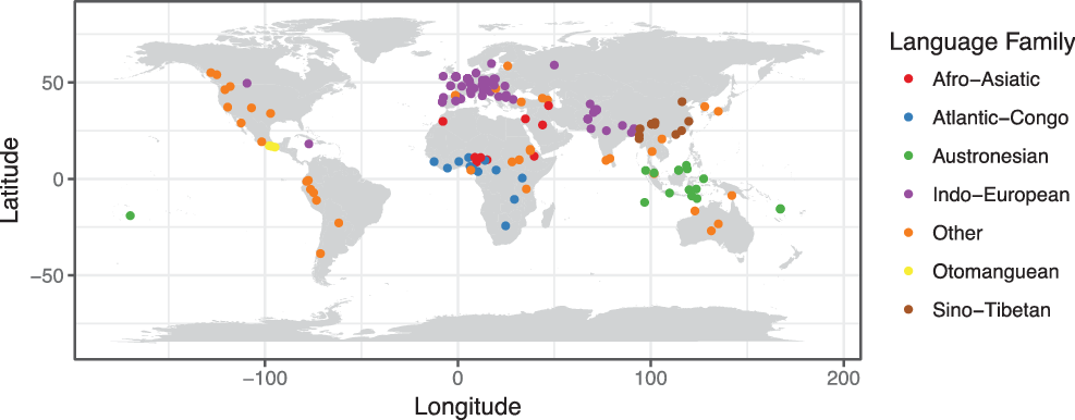
Figure 2 Map of languages in JIPA Illustrations. Language families with more than three languages in the corpus are colour coded.
A concern with our findings is that there is a non-trivial number of residual errors after tidying up the data: symbols that occur in the Illustrative Texts, but do not occur in the phoneme inventories (Figure 1d). The majority of these appear to be typos or data-entry glitches of the type discussed above. Almost half of the languages (45.6%) have at least one unexpected segment token in their transcripts. Of the languages that have these unexpected segment tokens, the average number in the transcript is three (s.d. = 9.5) and ranged from one to a maximum of 56.
Fortunately, while there may be a large number of unexpected segments tokens seen in a given language, these tend to be multiple observations of a small number of different segments. There was an average of two unexpected segment tokens in each language (of those that contained unexpected tokens), with a standard deviation of 1.7 (range = 1–8).
5 Transcript coverage
To analyse these data for coverage and recovery rate we implemented a series of custom scripts using Python (v3.5). We used these scripts to parse the inventories, and tokenise the transcripts into phonemes. To calculate the coverage of each inventory from the NWS transcript, we considered a phoneme as present if any of its allophones was observed in the transcript. For example, if the language had the allophones ‘a(a, a:)’ and ‘a:’ is found but not ‘a’, then the phoneme /a/ is still considered as recovered. Note that, while our approach here considers a phoneme as captured when only one of its allophones is observed, in practice a linguist would need to collect enough data to capture all allophones in their contexts, which means that our recovery times estimates are a lower bound estimate and capturing the allophone inventory would require more data. Any segments that were present in the transcript, not listed in the author’s inventory, but plausibly assignable to allophones based on our best available understanding, were added to the inventory and counted as recovered.
Languages are statistically non-independent due to their evolutionary relationships within language families and subgroups (Tylor Reference Tylor1889, Levinson & Gray Reference Levinson and Gray2012, Roberts & Winters 2013). For example, in terms of our data, perhaps certain language subgroups are more likely to share other aspects of language that might make it harder or easier to recover phonemes, or some other non-random effect. We used a Phylogenetic Generalised Least Squares (PGLS) regression to estimate how well the number of unobserved phonemes was predicted by the size of the phoneme inventory or the length of the transcript, while controlling for any effect of phylogeny. We extracted the accepted language classifications from the Glottolog database (v3.1; Hammarström et al. 2017), and used these to construct a language phylogeny using TreeMaker (v1.0; Greenhill Reference Greenhill2018), assigning dummy branch-lengths using Grafen’s (Reference Grafen1989) transform implemented in APE (v3.4; Paradis & Strimmer Reference Paradis, Claude and Strimmer2004). The phylogenetic GLS was fitted to this classification tree with the R library caper (v.1.0.1; Orme et al. Reference Orme, Rob, Gavin, Thomas, Susanne, Nick and Will2018) while adjusting for the error in branch-length information by the maximum likelihood estimate of Pagel’s λ (Pagel Reference Pagel1999).
The median number of unobserved phonemes in the transcript for each language was 7 (Figure 1c). The number of absences varied considerably, with a standard deviation of 9.7, ranging from a minimum of zero absences to a maximum of 53 absences. There are only three languages with perfect coverage (zero absences) in the JIPA Illustrative Text corpus: Shipibo, containing 24 phonemes (Valenzuela etal. Reference Valenzuela, Piñedo and Maddieson2001), the Treger dialect of Breton (Hewitt Reference Hewitt1978) with 36 phonemes, and Standard Modern Greek, containing 23 phonemes (Arvaniti Reference Arvaniti1999b). Therefore, only 3/158 of the languages have panphonic samples in the Illustrative text – 1.9%. The languages with the lowest levels of coverage were Estonian (Asu & Teras 2009) with 53/97 missing phonemes (largely due to under-sampling of its huge diphthong inventory), Hindi (Ohala Reference Ohala1994) with 45/85 missing, and Bangladeshi Standard Bengali (Khan Reference Khan2010) with 43/79 missing.Footnote 3
The relationship between the size of the phoneme inventory and the number of unobserved tokens (Figure 3a) was strong and significant (F(1,156) = 905.80, p < .0001) with an R2 of 0.85, and the number of unobserved phonemes was –15.52 + 0.64 (phonemes): as one would expect, the more phonemes a language uses, the harder it is to recover them (Figure 3a). Concretely, adding one phoneme to an inventory is expected to lead to another 0.6 phonemes remaining unobserved. In contrast, the number of unobserved phonemes was unrelated to the length of the NWS transcript (Figure 3b), as measured in number of segments (F(1,156) = 0.033, p = n.s.).

Figure 3 Relationship between (a) number of unobserved phonemes vs. inventory size and (b) number of unobserved phonemes vs. the length of the full Illustrative Text, measured in phoneme tokens. The orange line shows the significant phylogenetically controlled least-squares regression line, indicating the strength of the relationship.
Overall, these results indicate that the relationship between absences and inventory size was extremely strong: languages having larger inventories show more absences. On the other hand, the actual length of the transcript has a minimal effect on the phonemes observed. This lack of effect for total transcript length is presumably an outcome of the rapid observation of phonemes in the early sections of the transcript followed by a long slow decline in the observation rate (discussed below; see also Figure 5). The strong relationship between inventory size and unobserved phonemes in the transcript can be interpreted such that, for every phoneme added to the inventory, 0.6 extra phonemes are likely to be absent from the Illustrative Text.
There are 8/158 transcripts in the Illustrations corpus that do not use the ‘North Wind and the Sun’ narrative. These are Amarasi (Edwards Reference Edwards2016), Bardi (Bowern, McDonough & Kelliher Reference Bowern, Joyce and Katherine2012), Greek Thrace Xoraxane Romane (Adamou & Arvaniti Reference Adamou and Amalia2014), Nivaĉle (Gutiérrez Reference Gutiérrez2016), Nuoso Yi (Edmondson, Esling & Ziwo Reference Edmondson, Esling and Lama2017), Nuuchahnulth (Carlson, Esling & Fraser Reference Carlson, Esling and Katie2001), Spokane (Carlson & Esling Reference Carlson and Esling2000) and Taba (Bowden & Hajek Reference Bowden and John1996). One possibility is that authors have selected these alternatives because they better describe the language than the NWS narrative does; however, a one-tailed Kolmogorov–Smirnov test showed that there was no significant difference in the number of unobserved phonemes: D(0.16), p = n.s. However, this test is hardly robust given the small sample size (n = 8). A more robust alternative method for assessing the effect of different text sizes is provided by the simulation below.
6 The nature of phoneme frequency distributions
What type of frequency distribution is found in phoneme data? This question is of vital relevance to projections of how long a sample is needed to capture all the phonemes of a language. One possibility is that the frequency with which phonemes are observed in languages follows Zipf’s law (Zipf Reference Zipf1932, Reference Zipf1936; Piantadosi Reference Piantadosi2014). If the law does hold then the implications for recovering the phoneme inventory of a language are grim: by their very nature, power laws are ‘scale-free’ and therefore each new observation of data from a system generated by a power law process can give rise to novel entities. In short – if phoneme frequencies follow Zipf, we will never get all the phonology according to Rhodes et al.’s criteria above, and the answer to the Bird–Himmelmann problem is ‘never’. As such, the inventories published in JIPA would therefore be simple samples of the most frequent phonemes in the corpus studied by the authors of the Illustration.
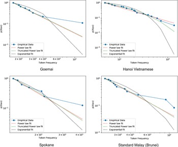
Figure 4 The complementary cumulative distribution of segment token frequencies in four randomly selected languages. The attested frequencies are plotted in blue, while the fit of three candidate distributions are indicated with dashed lines. The y axis, ‘p(X ≥ x)’ is the probability of observing a phoneme X with the frequency less than or equal to x.
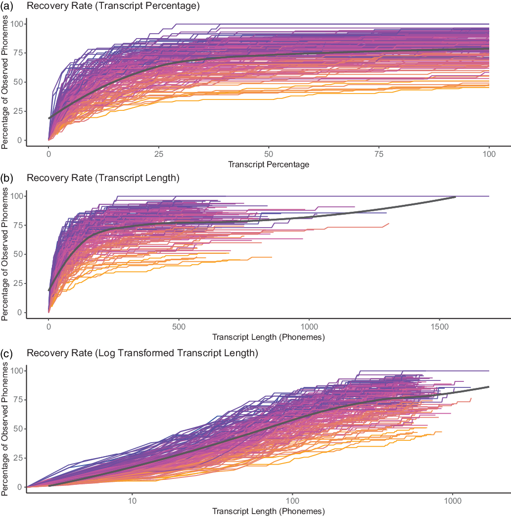
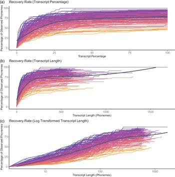
Figure 5 Rate at which a language’s phoneme inventory is recovered in the NWS transcript. Individual languages are coloured by the size of their respective inventories: (a) shows the recovery rate as a function of transcript percentage, while (b) shows the recovery rate as a function of transcript length, and (c) shows the rate in (b) transformed into a log scale. The black lines are local regression ‘LOESS’ curves fitted to the data.
To evaluate whether phoneme frequencies followed a Zipfian power law distribution we calculated, for each language, the frequency of each phoneme in the transcript. Using the powerlaw python library (v1.4.3; Alstott, Bullmore & Plenz Reference Alstott, Bullmore and Plenz2014) we evaluated the best fitting distribution by comparing log-likelihood ratios between four different candidate distributions:
-
1. a power law;
-
2. an exponential distribution (not a power law, but has a thin tail with low variance);
-
3. a log-normal distribution (not a power law, but has a heavy tail);
-
4. a truncated power law (which follows power law behaviour over a certain range, but has an upper bound given by an exponential).
To test whether phoneme frequencies follow a Zipfian distribution, we first fitted a power law distribution to the frequency of each language’s phonemes, and calculated the value of the scaling parameter a. If these distributions are Zipfian, then a should approximately equal 1 (Piantadosi Reference Piantadosi2014). However, the estimated a values have a median of 1.38 and a standard deviation of 0.052 (range = 1.25–1.54) and do not overlap with the expected a of 1.
As a more rigorous and formal test of whether Zipf holds for the phoneme frequencies, we compared the fit, for each language, of three other candidate distributions (power law, exponential, log-normal, and truncated power law) to that of a power law using a log-likelihood ratio (Clauset, Shalizi & Newman Reference Clauset, Cosma Rohilla and Newman2009, Alstott et al. Reference Alstott, Bullmore and Plenz2014). Formally, significance was assessed using a log-likelihood ratio, R, normalized by its standard deviation:
 $\textrm{R}/(\sigma\surd\textrm{n})$
, where more negative values show stronger support for the alternative distribution. The truncated power law distribution was a significantly better fit than the power law for 150/158 (95%) languages, while the other eight (5%) languages were significantly better explained by a log-normal distribution, and the average normalised log-likelihood ratio difference between the power-law distribution and the best fitting model was large (median = –6.70, s.d. = 2.76, range: from –2.26 to –17.75). However, visual inspection of cumulative distribution plots of the model fits reveals that, while the truncated power law was the best fitting model, there were often substantial deviations from this model, especially towards the tail, suggesting that the truncated power law is not a good approximation of the true frequency distribution.
$\textrm{R}/(\sigma\surd\textrm{n})$
, where more negative values show stronger support for the alternative distribution. The truncated power law distribution was a significantly better fit than the power law for 150/158 (95%) languages, while the other eight (5%) languages were significantly better explained by a log-normal distribution, and the average normalised log-likelihood ratio difference between the power-law distribution and the best fitting model was large (median = –6.70, s.d. = 2.76, range: from –2.26 to –17.75). However, visual inspection of cumulative distribution plots of the model fits reveals that, while the truncated power law was the best fitting model, there were often substantial deviations from this model, especially towards the tail, suggesting that the truncated power law is not a good approximation of the true frequency distribution.
7 Recovering the full phoneme inventory
Plotting the rate at which the phoneme inventory is recovered from the Illustrative Text transcript gives us the curves shown in Figure 5. This figure demonstrates that the recovery rate varies substantially between languages, as expected given the strong relationship between the number of unobserved phonemes and the size of the phoneme inventory.
Many of the phonemes are identified quickly. Half the phoneme inventory is identified within a median of the first 20% (s.d. = 25.91%) of the NWS transcript (or a within a median of 112.5 segment tokens, s.d. = 121.5). After this initial rapid burst of recovery, the rate at which new phonemes are found in the transcripts rapidly declines. For example, the phoneme /ʒ/, which is the rarest of English phonemes, will only begin to appear when words like usual (frequency rank order #304) or measure (frequency rank order #323) appear (http://www.rupert.id.au/resources/1000-words.php). This relative rate of decline happens faster as the size of the phoneme inventory increases. This overall rapid decline in recovery rate can be seen from the black local regression curves (LOESS) fitted onto Figure 5 which rapidly plateau out to a much slower rate of increase. On average the second half of a transcript only contains a median of 2 previously unobserved phonemes (s.d. = 1.9).
To assess how much data is needed to recover all the phonemes of a language we developed three different approaches: (i) LM (Linear Model), (ii) Generalised Additive Model (GAM), and (iii) Simulation.
The first method attempts to model the rate of phoneme recovery of time to extrapolate to complete recovery. Here we apply a LM to model how the percentage of phonemes observed increases with the logged amount of text observed. We regressed the logged text length on the observed phoneme percentages at each point in the transcript (i.e. the relationship in Figure 5c). We transformed the amount of observed text using a log10 transform as the recovery rate curves tended to follow a truncated power law distribution (see Figure 5), and used a Poisson log-link function in the regression. We then used the observed relationship to predict the amount of text required when the percentage of observed phonemes was 100%.
While the LM is a relatively simple approach, visual inspection of the log10 transformed recovery rates and residuals suggested that the relationship between logged text length and the percentage of observed phonemes could be non-linear, and the residuals for many languages contained homoskedasticity (i.e. unmodelled trends). Therefore our second approach applies a Generalised Additive Model to the same log10 transformed data. The GAM method fits a series of curves to the relationship, allowing the best fit estimate to incorporate non-linearity (Winter & Wieling Reference Winter and Martijn2016). Here we used thin plate regression splines – i.e. we approximated the curves with a series of lines – to model the relationship following Wood (Reference Wood2011). To avoid over-fitting the curves we set the maximum number of knots to be low (k = 8) as visual inspection of fitted curves and checks of the residuals indicated that at higher k’s the fitted curve became very flat for the last few data points, leading to the estimated time for complete recovery ballooning to millions of tokens for some languages.
The LM and GAMs were fitted to each language using R (v3.5.0; R Core Team, 2018) and the package mgcv (v1.8-23; Wood Reference Wood2011, Reference Wood2017). All graphs were plotted using ggplot2 (v2.2.1; Wickham Reference Wickham2009).
The two modelling approaches LM and GAM are, however, heavily contingent on the narrative used – the phoneme observation rate is shaped by the narrative constraints of the ‘North Wind and the Sun’ story in that language (e.g. there are multiple repetitions of the phrase ‘North Wind’ and its constituent phonemes), as well as morphosyntactic flow-on effects (e.g. the fact that it is a past-tense narrative, rather than a procedural, inflates the number of past-tense suffixes (-əd/-d/-t in the Australian English version). One approach to inferring a more general figure of the amount of data required would be to identify alternative phonetically encoded corpora and compare their time to recovery; however, these corpora are rare and would require the phonemic transcription to match the JIPA paper. Another approach would be to shuffle the words of the JIPA narratives and infer different recovery rates. However, these shuffled texts would be only superficially different as the phoneme frequencies would remain the same (i.e. there would be the same number of schwas, just in different orders).
Therefore we developed an alternative simulation approach to mimic the process of sampling different texts and thus infer how different texts might affect the total recovery time. Here we assume that the frequency of phonemes in the ‘North Wind and the Sun’ approximates the real frequency with which phonemes occur in the language, but is not constrained by the narrative or even the morphosyntactic structure of the language. Thus each simulated text is informationally nonsensical; however, it is not as constrained by the narrative information in the ‘North Wind and the Sun’. Conceptually each random text should be phonemically similar to a real text with randomly shuffled phonemes. Importantly, the simulation approach allows the observations of phonemes to vary probabilistically, which allows us to estimate the average text length per language and the associated uncertainty around that estimate.
To make this simulation we need to calculate the probability of seeing each phoneme in each language. It is easy to calculate the observation probability for each phoneme observed in the Illustrative Text, but the observation probability for phonemes that are never seen is zero. However, we can estimate the probability of the unseen phonemes using a common statistical approach: Good–Turing frequency estimation (Good Reference Good1953, Gale & Sampson 1995). This approach calculates the frequency of frequencies of phoneme observations (i.e. how often have we seen any phoneme n times). The probability for unobserved phonemes is then set to the number of times phonemes have been seen once, and the observed phonemes are rescaled down such that the full probability distribution sums to 1. We used the ‘Simple’ variant of the Good–Turing smoothing algorithm implemented in the python library Natural Language Toolkit (NLTK v3.3; Bird, Klein & Loper Reference Bird, Klein and Loper2009). In each simulation we sample phonemes from this distribution randomly to generate a random text until we have seen that language’s full inventory. For each language we repeated this process 1000 times to get an estimate of the median text length (and standard deviation) required.
There are two provisos with this simulation. First, the Good–Turing smoother requires hapaxes (observations seen once) to approximate the probability of unseen tokens. When a language had no hapaxes, we subtracted 1 from each observed token, essentially scaling down the distribution until it did contain hapaxes. This affected 11 languages. Second, where a language had no unobserved tokens remaining to be seen, the specific implementation we used in NLTK required the addition of one extra dummy token which will mildly underestimate the observation probabilities and subsequently lead to a minor overestimation of the required time to capture the language. This only affects the identified languages with complete capture (Standard Modern Greek, Breton (Tregar), and Shipibo).
8 Evaluating the methods against a larger corpus
Our findings in the preceding section suggest that Zipf’s law does not hold for phonemes. Rather, the number of phonemes in these languages are best described by a truncated power law distribution which does have a finite ending point. Admittedly, our results are based on a very small corpus for each language and there are estimation issues on small datasets (Clauset et al. Reference Clauset, Cosma Rohilla and Newman2009), so this finding must be taken as indicative only. However, the finding is consistent with previous work on larger corpora showing that phoneme frequencies follow other distributions (Sigurd Reference Sigurd1968, Martindale et al. Reference Martindale, Gusein-Zade, McKenzie and Borodovsky1996, Tambovtsev & Martindale Reference Tambovtsev and Martindale2007). While the power law behaviour is true of lexica – one can always create a new word – it is hardly likely to be true of phonemes which, we presume, need to be present at a certain frequency in order to have a hope of combining into words offering the minimal pairs that ensure their contrastive status as a phoneme.
That makes it imperative to get a realistic estimate of what curve works best, based on a larger corpus size. To this end, we carried out an additional examination of the growth in capture rate across a much longer text – the Bible. Fortunately, the JIPA corpus contained one language with a fully phonemic orthography with a one-to-one phoneme to grapheme mapping and multiple Bible translations, namely Czech.
Using a parallel text corpus (Mayer & Cysouw 2014) we obtained phonemically transcribed Bible translations for Czech: 7 bibles, average tokens per bible = 3,290,304 phonemes. (In fact these bibles included three graphemes/phonemes beyond the set used in the JIPA Illustrations (namely /ɛu/, /oː/, and /au/), a fact that will become relevant below.)
We calculated recovery rates using these bibles (with a different rate plotted for each individual bible) and found recovery rate curves closely similar to the ones we obtained from the JIPA Illustrations (Figure 6). The rate at which phonemes are recovered in the bibles is rather similar to the rate at which they are recovered in the JIPA Illustrations, but in fact rises more slowly. This consistency of recovery rates across different corpora suggests that our approach to calculating the amount of text required for full recovery would give similar results if conducted on much larger corpora than the JIPA narratives.

Figure 6 Consistency of recovery rates for the phonemic orthography in Czech (Log Scale for Number of Tokens Observed). The line in blue indicates the recovery rate found in the JIPA Illustration, while the lines in red indicate the recovery rates for the same languages in large bible corpora.
Since the Czech bibles are much longer texts, they do fully recover the phoneme inventory (Figure 7). Strikingly, the amount of text required to capture the full inventory varies substantially across the different bibles, ranging from 6202 segment tokens (Novakarlica bible) up to 80,959 tokens (New World bible). On average the number of tokens required was a median of 68,084, with a substantial standard deviation of 34,680. This variation indicates a major dependence on the text used as an example – and note that the variation in recovery rate primarily affects the low-frequency phonemes, as the pattern of high-frequency phonemes appears to be relatively consistent across texts (see Figure 6). In contrast, the identification of low-frequency phonemes is heavily contingent on sporadic word choices. For example, in these bibles the final few phonemes to be captured are /ɛu/, /oː/ and /au/, and these largely occur only in low-frequency words like Eufrat ‘Euphrates’, Nód (i.e. the Biblical land of), and Ezau (the older son of Isaac).
We can now use this ‘real’ count of the number of segment tokens required to evaluate how accurate our three methods of estimation are. To do this, we calculated the recovery rate curve for each bible separately (i.e. Figure 6). As the JIPA Czech Illustration does not include the last three phonemes to be captured (namely /ɛu/, /oː/ and /au/) we also truncated the bible texts to the same point, i.e. to the point where all but these phonemes had been captured. Then we estimated the number of tokens required from these truncated curves using the LM, GAM and Simulation approaches. The results are shown in Figure 7. The most accurate method was the Simulation approach, which included the real estimate within the simulated range for all bibles, and placed the real estimate at the centre of the estimated distribution in four out of seven cases. In the other three cases, the real estimate is near the upper extremes of the distribution, suggesting that the Simulation approach provides a slightly conservative estimate of the real amount of text required. In contrast, the LM and GAM approaches heavily underestimate the real amount required. Further, as the Simulation approach provides a measure of amount of text required, this mimics the variation seen in phoneme recovery rates across the different bibles. Therefore, we suggest that the best method here is the Simulation approach and use it as the primary focus in the discussion.
9 Returning to the cross-linguistic data
Armed with this finding, we now return to the cross-linguistic data. In all three approaches the number of segment tokens needed to fully describe a language’s phoneme inventory varied substantially (Figures 8 and 9). Under the LM approach the number of segment tokens needed for full recovery was a median of 1026 tokens (s.d. = 51,657) and ranged from a minimum of 256 to 446,227 tokens, according to the language.Footnote 4 The GAM approach implied a similar amount with a median of 1182 (s.d. = 579,830) and minimum of 275 tokens; however, this model increased the higher end of the distribution by an order of magnitude to 7,126,644 tokens. These extreme values occurred in the Hindi, Telugu and Bengali (Bangladeshi Standard) languages, which have some of the lowest rates of phonemes captured in the NWS transcript (47%, 48% and 45% observed respectively), coupled with low rates of recovery. Our preferred method, the Simulation approach, does not find the same long tail. Instead the median text length for recovering a full phoneme inventory in the Simulations was 3278 segment tokens (262 seconds, about 4.5 minutes) with a substantial standard deviation of 8059 (Figure 8). The minimum number of segment tokens needed to fully describe a language’s phoneme inventory varied from a minimum of 87 tokens to a maximum of 145,010 tokens.

Figure 7 Comparison of recovery methods on various Czech bibles. Black cross shows the real number of tokens needed to fully capture the full inventory. The blue and orange points show the estimated number of tokens from the LM and GAM methods respectively. The cloud of grey points shows the estimate from the simulation method where each point is a single simulation.
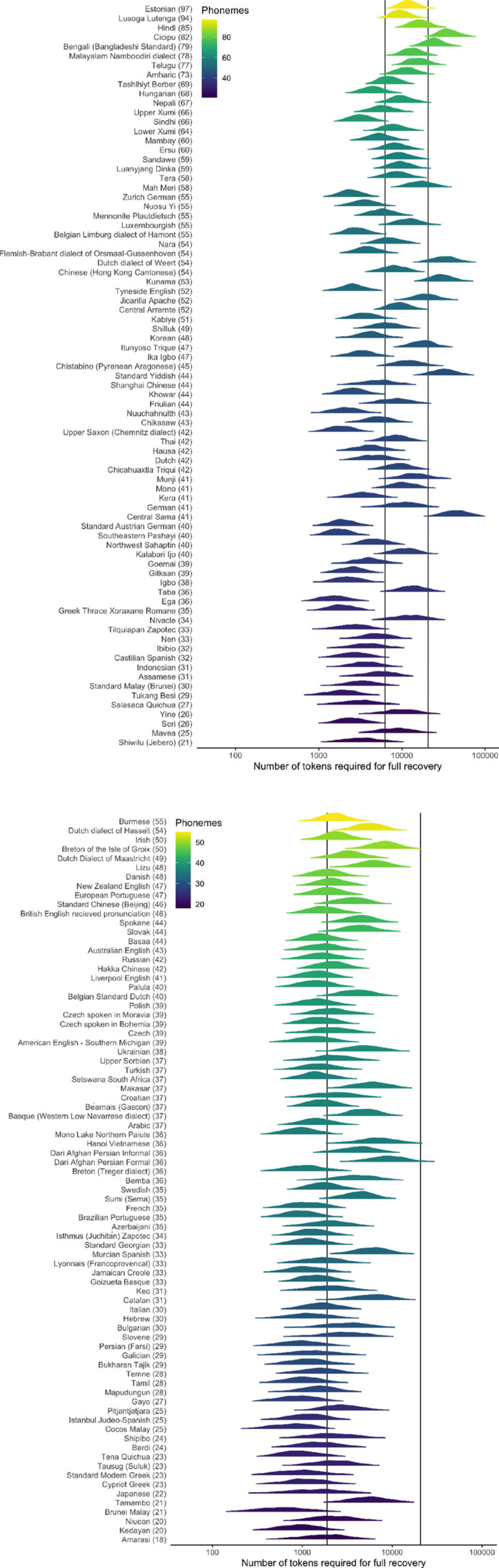
Figure 8 Estimated number of segment tokens needed to fully recover a language’s phoneme inventory under the Simulation approach. Languages are ranked by number of phonemes in their inventory from largest (top) to the smallest (bottom). The first vertical line indicates the median number of tokens required, while the second indicates the number of tokens required to capture 95% of the simulated language texts.
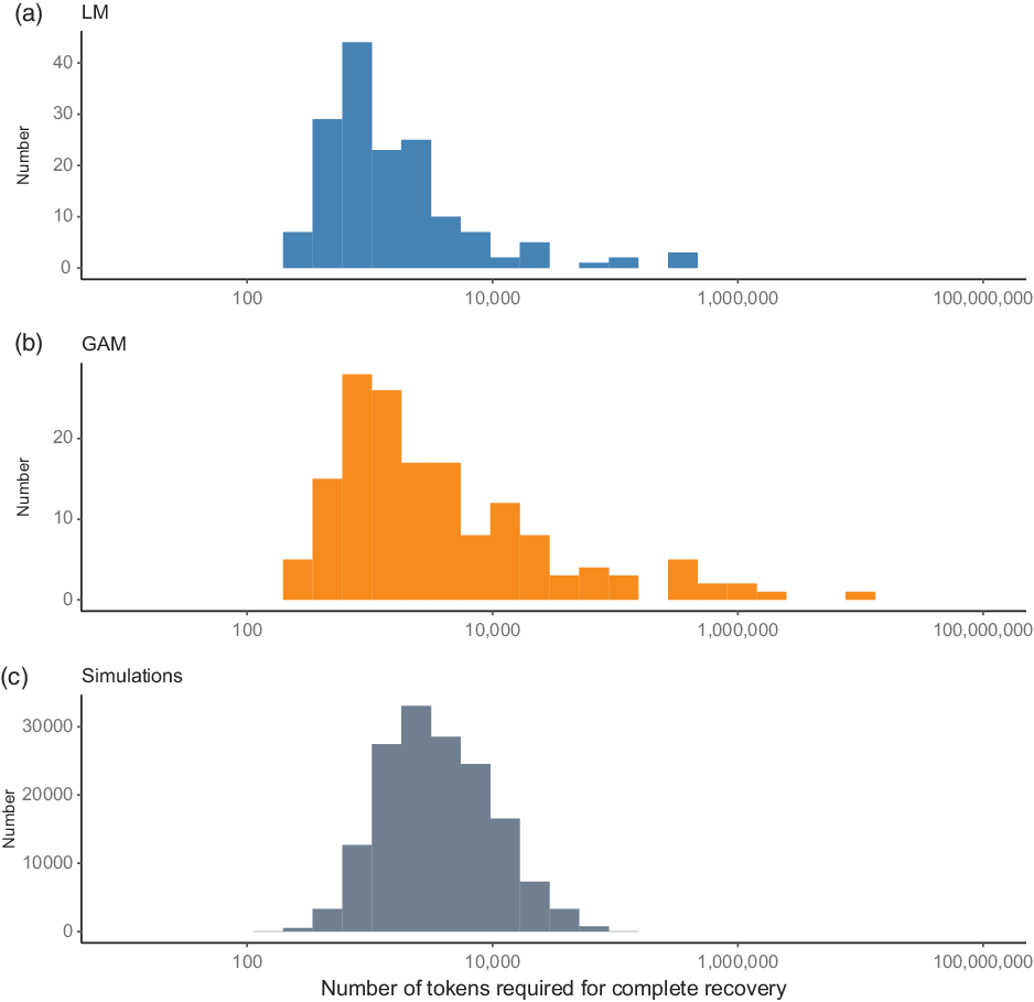
Figure 9 Histogram showing the overall amount of text needed for full recovery of a phoneme inventory across all languages using the three methods.
The results from all three methods are strongly correlated (LM vs. GAM Spearman’s ρ = 0.87, p < .0001, LM vs. Simulation ρ = 0.77, p < .0001, GAM vs. Simulation ρ = 0.73, p < .0001). Under the LM method the languages with the fastest recovery were Kedayan with 256, Persian (Farsi) with 263, and Standard Modern Greek with 271 required tokens respectively, while the GAM found Persian (Farsi) with 275, Standard Modern Greek with 285, and Galician with 290 required tokens. The worst-case scenario languages were the same in both analyses: Hindi (LM = 446,227, GAM = 7,126,644), Telugu (LM = 331,600, GAM = 1,325,217), and Bengali (LM = 291,054, GAM = 909,283). With the Simulation method the languages with the fastest full recovery were Brunei Malay (recovered after 87, 111 and 114 tokens), Japanese after 112 tokens, and Cocos Malay after 115 tokens. The worst-case scenario languages were Central Sama (with the slowest simulation needing 145,010 tokens), Standard Yiddish (112,628 tokens), Cicipu (109,956), and Kunama (105,427). A full 95% of the simulated datasets were captured after 20,674 tokens (or 23,556 tokens in the LM and 38,7326 in the GAM approach), i.e. 1650 seconds, around 27 minutes of text.
There is a concern with some of the simulation estimates that should be kept in mind. The Good–Turing smoothing algorithm used for these simulations approximates the probability of low-frequency states using a linear regression (Gale & Sampson 1995). This regression is used to estimate the probabilities when the variance on the Good–Turing smoother becomes unpredictable (i.e. exceeds two standard deviations). Gale and Sampson note that probability estimates may become unreliable if the slope of this regression is greater than –1. The distribution of slopes had a median of –1.08, with standard deviation of 0.21, and therefore some of the slopes estimated for the languages were indeed larger than –1 (n = 56). However, we feel this is not a major issue here, for two reasons. First, most of the inferred slopes were smaller than the threshold of –1 (n = 99/157). Second, this slope is only used to smooth the estimate of the low-frequency states and in all of these problematic cases the switching time between the Good–Turing smoother and the linear smoother was identified at frequency counts of 1. Therefore, the regression estimate was only used to estimate the frequency of singletons (hapaxes) and absences in a third of the simulations. The net effect of flattening the regression slope will be to underestimate the probabilities of these segment tokens and make our estimated recovery times more conservative. In addition, the median amount estimated by the simulation method for each language was highly correlated with both the results from the LM (ρ = 0.77, p < .0001) and GAM (ρ = 0.72, p < .0001) approaches.
As can be seen in Figure 8, there is a relationship between the size of a language’s phoneme inventory and the number of tokens required to capture the inventory. To quantify this we conducted another PGLS to predict the required number of segment tokens (as estimated by the Simulation approach) for full recovery based on the number of phonemes in any given language. As there was a non-linear relationship between number of segment tokens and phonemes, we transformed the dependent variable with a log transform (i.e. a log-linear regression). A significant relationship was found (F(1,156) = 82.76, p < .0001) with an R2 of 0.35 such that log(Recovery Length) = 2.887 + 0.0165 × Inventory Length. Therefore, for every phoneme added to the inventory, the amount of text required to observe it increased by 1.67%. However, Figure 8 also indicates that, while there is an effect of the phoneme inventory size in increasing the amount of text required, the worst-case languages are not necessarily the ones with the largest inventories – instead this must be linked to the interaction between inventory size and the frequencies of the tokens in the original text. Future work should explore this in more detail.
10 Estimating the amount of audio needed
To estimate how much audio is needed to recover all phonemes in a language we obtained the audio length in seconds from the Illustrations which had recordings of the ‘North Wind and the Sun’ narrative, after excluding those with dysfluencies or side passages. When a language had multiple versions of a recording (e.g. from different speakers), we estimated the average time across all versions. We then estimated the average time per segment token for each language by dividing the audio length by the number of segment tokens in the transcript. Finally, to estimate the time to fully recover the phoneme inventory we converted the estimate of required text length to time by dividing this by the time per token.
The mean time for a phoneme in our languages ranged from 0.039 seconds in Hong Kong Cantonese to 0.201 seconds in Gitksan. The median time per phoneme was 0.080 seconds with a standard deviation of 0.0286 seconds. Under the Simulation approach, the required text length for full phoneme inventory recovery was a median of 261.79 seconds (s.d. = 694.94 s). The fastest languages to be captured were Brunei Malay with a median of 37.9 seconds, followed by Standard Modern Greek (median = 43.8 s) and Cypriot Greek (median = 54.7 s). The languages that took longest to be captured were Cicipu (median = 4040 s), Central Sama (median = 3312 s) and Kunama (median = 2573 s). However, the distribution of estimated times is right-skewed, and while only a small proportion (∼1%) of simulations require more than one hour of recorded text, these outliers are heavily concentrated in a small subset of the languages: Cicipu (68.30% of the simulations required more than one hour), Central Sama (41.60%), Kunama (16.00%), Bengali (Bangladeshi Standard) (6.60%), Dutch dialect of Weert (5.40%), Mah Meri (5.20%), Munji (0.60%), Kalaḅarị-Ịjọ. (0.30%), Mavea (0.20%), Nivaĉle (0.20%), Makasar (0.10%), and Yine (0.10%). If we remove these outliers then the average amount of time to completely recover a language’s phoneme inventory was 257.75 seconds (s.d. = 532.53 s). For 98.94% of the languages the full inventory can be recovered in less than an hour’s recording, on all simulations. However, if we adopt the most conservative ‘ready for anything’ approach, and including all simulations across all languages, so as to take in our worst-case scenario (one of the Cicipu simulations), we need nearly three and a half hours (12,445 seconds = 3 hours and 27 minutes).
11 Effect on recovery of cross-linguistic frequency/rarity
As shown in the preceding sections, many sampling procedures, unless they are much longer than usually employed in JIPA Illustrations, will fail to capture some number of phonemes. In this section we look at how serious this problem is, by asking how the cross-linguistic frequency of phonemes interacts with the likelihood of being missed in sample texts. To understand why this matters, take a phoneme that is found in only a handful of languages. If this phoneme is relatively frequent within that handful, then our attempt to fully describe the world’s languages is lucky as we will quickly observe many tokens of the rare sound. However, if the rare phoneme is also rare in the languages where it does occur, then the attempt to fully document global phonetic diversity has a high risk of missing true phonemes that just happen to occur in a few languages with low frequencies.
To investigate this issue we collected the top 250 most commonly occurring sound segments listed globally using the PHOIBLE database (Moran, McCloy & Wright 2014). We removed all tones from the list to be consistent with our study and added the next 12 items to make the list up to 250 items. We then matched these phonemes to the ones observed in the JIPA Illustrations. For each phoneme we calculated three measures from the combined PHOIBLE and JIPA Illustration data. The first measure is the global phoneme rank, i.e. how common the phoneme is in all the languages in the global sample in PHOIBLE. The second measure calculated the frequency of each phoneme in the languages in the JIPA sample. The third measure was the percentage of the transcript elapsed before the first time a given phoneme was seen, averaged across all languages in the JIPA sample. This third measure essentially measures the average number of tokens we need to see before we observe an instance of this phoneme.
Figure 10 shows the relationships between the average percentage of the NWS text needed to observe a phoneme and the global ranking and JIPA frequency. First, the global frequency of a phoneme and the time it takes to capture that phoneme is moderately correlated (ρ = 0.46, p < .001). This moderate relationship also holds, to a slightly stronger degree, when we look just within the JIPA Illustrations (ρ = 0.55, p < .001). Intriguingly, the most common 50 phonemes globally are almost all observed within the first 25% of the transcript, while there is a long tail of phonemes that take substantially longer to find. As we have already seen, some phonemes are never observed, even after the complete transcript (coloured red in Figure 10 at 100% on the x-axis), and, worryingly, these are predominantly the rarer phonemes. This gap is most noticeable in calculating rarity by frequency in the listed JIPA Illustration inventories, but even using the global ranking we see that none of the world’s top 50 phonemes are missed when they should be present.
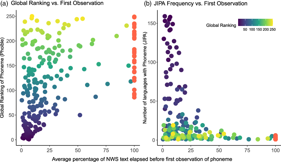
Figure 10 Scatter plots showing the relationship between (a) the global ranking of each phoneme, and (b) the frequency of each phoneme within the JIPA Illustrations, compared to the average percentage through the transcript of the phonemes’ first observation. The colours indicate the global ranking of how common the phoneme is according to PHOIBLE, with bluer points being found in the top 50, and yellower points found less frequently. Points coloured in red are the phonemes that are not observed after the complete transcript.
In short, rarer phonemes, on average, require more data for us to observe them. The rarest sounds globally are also the rarest sounds within an individual language’s sound system. Phonemes that are found in more languages are more likely to be seen in the transcripts, while the world’s rarer phonemes are less likely to be seen, and hence captured in an Illustration. This is problematic for the value of NWS texts, since the rare phonemes are the very ones that are most necessary if we are to describe the world’s phonetic diversity fully. Yet they are the ones less likely to occur in the NWS texts.Footnote 5
12 Discussion
The results presented here have implications for future Illustration papers, shed light on the Bird–Himmelmann problem, and raise several unresolved issues for future work.
12.1 Recommendations for JIPA
Through the process of coding languages, the difficulties involved in typographical accuracy became very apparent. While we are sympathetic to authors, more careful checking needs to be carried out at different points in the publication process. Authors need to be aware of the kinds of errors that are likely to appear in their transcriptions, and therefore be vigilant when proof-reading. (For example, the more diacritics are used, the more typographical errors there are.) Editors need some kind of mechanism – preferably automated – for checking that every symbol in the transcription is accounted for in the body of the Illustration, either in the phoneme inventories, or in the discussion. Then, consistency between the phoneme inventories, discussion and the transcription needs to be checked.
Despite the difficulties in correctly describing languages in the IPA and Illustrations format, we want to emphasise that this is still a deeply worthwhile endeavour. This paper is a case in point – it is only due to the unprecedented collection of material formed by the pooled Illustration papers that we are able to tackle important questions like those raised by Himmelmann and Bird. One plea is that this corpus needs to include a wider range of non-European languages.
One supplementary method for overcoming the power-law problems discussed in the preceding section would be to include panphonic texts in future JIPA Illustrations, or even for authors to consider modifying the NWS text that they collect in a way that renders it panphonic. Discussion concerning the gaps left in the coverage of phonemes by the NWS text is not new. Deterding (2006) suggested using the story ‘The Boy Who Called Wolf’ as a replacement for ‘The North Wind and the Sun’, after identifying its limitations for the description of varieties of English. Jesus, Valente & Hall (2015) explored whether the NWS text was panphonic (or in their terminology ‘phonically balanced’; 2015: 2) for European Portuguese and Brazilian Portuguese, and evaluated its suitability to be used as a panphonic text in, for example, clinical settings. Their conclusion was that ‘The BP [Brazilian Portuguese] transcription covers all phonotactic rules, but does not present all phonemes’ (2015: 9), while the European Portuguese version ‘covers all phonemes and all phonotactic rules in EP [European Portuguese], and is balanced in frequency’ (2015: 9).
Hiki, Kakita & Okada (2011) have shown that the NWS text can be made panphonic for Japanese. They created an alternative panphonic version of the NWS text for a JIPA Illustration with the purpose of providing ‘a more complete set of consonant phonemes and their allophones for the Illustration of the IPA of Japanese speech sounds’ (2011: 873). While their knowledge of Japanese phonology informed the creation of this panphonic text, their analysis of phonemes and allophones was then based on the text, drawing on textual examples. In order to create a panphonic text, they searched for appropriate synonyms and avoided onomatopoeic, mimetic, conversational expressions and loan words (2011: 872). The panphonic version of the text is, the authors say, 30% longer than the Japanese version of the Illustrative Text (2011: 872), although what unit was measured to obtain the 30% figure is unclear. However, they state that it took one minute to read ‘with an average speech rate’ (2011: 872), which is in contrast to the 32 seconds for the JIPA published version.
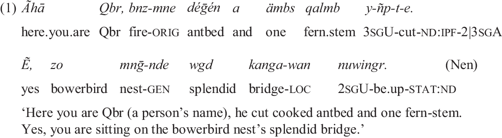
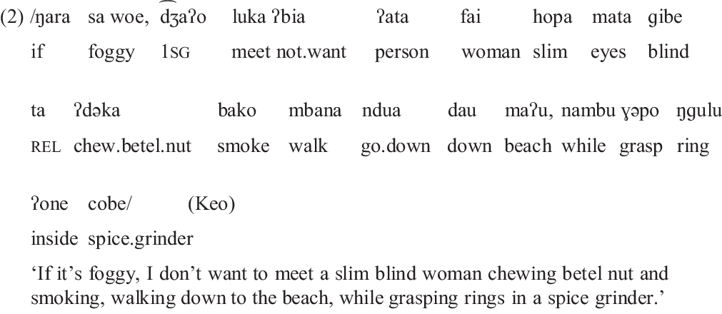
An alternative to producing a panphonic version of the ‘North Wind and the Sun’ text in each Illustration may be for a short supplementary panphonic text to be provided. We here provide examples for two languages for which JIPA sketches have been previously published, namely Nen (a Papuan language, spoken in Southern New Guinea), and Keo (an Austronesian language, spoken on the island of Flores in Indonesia). The Nen example in (1) is written in practical orthography, which has a one-to-one phoneme–grapheme correspondence, except that schwas are not written in most word positions, while the Keo example in (2) is written phonemically, using the IPA.
12.2 How many data are needed to fully capture a language’s phoneme inventory?
Key to moving from our initial finding in Section 5, that most NWS texts fail to capture all phonemes, to an estimation of how much text would in fact be needed, is to fit a range of possible curves to extrapolate the growth in capture rate (Section 6) and from this to develop estimates of the necessary transcript length (Section 7). However, since the best-fit curve is underdetermined by the initial phases of growth, we went back and re-evaluated candidate curves (LM, GAM and Simulation) against a collection of longer (Bible) texts for Czech in Section 8, concluding that the best fit comes from a ‘simulation approach’ which mimics the process of sampling shuffling phonemes according to their real frequency in the language. Armed with that model we returned to our cross-linguistic data in Section 9, finally able to give concrete estimates of the number of tokens needed for complete capture across a range of languages, then converting that into time estimates in Section 10 using estimates of median time per phoneme extracted from the whole cross-linguistic sample.
Our results from these simulations sheds light on the Bird–Himmelmann problem as follows. First, each extra phoneme in a language provides a measurable documentary burden. Adding a new phoneme to a language increases the amount of text required for full recovery by 1.67% within the NWS story. Whilst this increase is small, it balloons rapidly. We estimate that the amount of text needed for full recovery for a language with an average sized inventory is 3,278 tokens – more than five times longer than the average length of the NWS Illustrative texts. As languages increase their phoneme inventories this limit increases too. We estimate that the full phoneme inventory of most languages (95%, using simulation) can be obtained after 20,674 tokens – almost 40 times larger than the average NWS Illustrative text. In the worst-case scenario, languages with extremely complicated phonologies could take more than 50,000–100,000 tokens to capture all the phonemes, though for nearly 99% of cases there is complete coverage inside an hour of material. Our worst-case projection, for Cicipu, was around three and a half hours (12,445 seconds = 3.46 hours). Though way longer than any NWS text, documentarists and funding agencies can take heart from the fact that even this worst of worst-case scenarios falls within the amounts of data being deposited by typical Ph.D. projects on previously undescribed languages.
It is important to note, however, that the JIPA Illustrations start from the presumption of a known phoneme inventory, where minimal pairs and other data types supplement that found in the NWS text. In general, we can assume that the minimal text length needed to establish a phonemic analysis exceeds that needed to deliver a representative of each phoneme, since establishing a phonemic analysis relies on minimal pairs, which generally involve word-length strings whose probability of occurrence is much lower than that of individual phonemes.
Our final point follows from our findings that cross-linguistically rare phonemes are less likely to be captured in language-specific NWS texts. One of the key goals of the JIPA Illustrations is to extend our knowledge of the world’s sounds, and illustrate how they should be notated. Yet it is precisely those sounds that are less likely to have been described before which are also least likely to appear in NWS texts. The need to get running-text exemplifications of these previously unreported sounds amplifies the point made earlier regarding the value of panphonic texts.
13 Conclusion
The study undertaken here does not aim at a complete answer to the Bird–Himmelmann problem. For example, the very low bar we have set for capture (one allophone of a phoneme being sufficient) means that full attestation of all allophones of all phonemes would require a substantially larger corpus. And remaining just in the phonology, other levels of coverage – attesting all minimal pairs needed to establish the body of phonological contrasts, or all clusters needed to fully specify the phonotactics, or all word structures needed to understand the metrical phonology, tone sandhi etc. – will all need larger corpora because each needs to combine all phonemes in some more complex way.
A further crucial point to note here is that the JIPA Illustrations start from the presumption of a known phoneme inventory, where minimal pairs and other data types supplement those found in the NWS text. The various elicitation methods employed by linguists in investigating a language’s phonology can be viewed as ways of accelerating the discovery process for phonological structure, for example, by probing which small differences in pronunciation stray into the allophonic range of another phoneme, or capitalising on what is known of the phonological structure of related languages to guess at and construct words likely to deliver minimal pairs. The measures we are interested in here are therefore not targeted at what is needed for phonological discovery, but rather for confirmation of distributions across texts not biased by the demands of elicitation, as well as for trialling other computational methods, such as machine-learning.
We can safely assume that the minimal text length needed to sample all allophones and environments needed for a phonemic analysis exceeds that needed to deliver a representative of each phoneme, since establishing a phonemic analysis relies on minimal pairs, which generally involve word-length strings whose probability of occurrence is much lower than that of individual phonemes. The wise words of Rhodes et al. (Reference Rhodes, Grenoble, Anna and Paula2006: 4) should be heeded here, to temper how the figures given here are interpreted:
How do we know when we’ve gotten all the phonology? When we’ve done the phonological analysis and our non-directed elicitation isn’t producing any new phonology.
Going further into other levels of linguistic organisation, since phonemes are the building blocks of words and their component morphological units, it follows that the sample size to get complete coverage for any of these domains will be much larger than that discussed here. And beyond that, many further types of crucial linguistic data – e.g. semantic ambiguities attaching to particular syntactic constructions, which by definition require more than one utterance (or interpretation thereof) with the same form – multiply the amount of material still further. For example, the ambiguity of Chomsky’s famous Flying planes can be dangerous, whose semantic ambiguity is paired with a syntactic ambiguity, would only be detected in a corpus if it occurred in two different contexts revealing the different meanings, or else was paired with a commentary by a speaker who noted the ambiguity.
There can thus be no single answer to the Bird–Himmelmann problem, since many different metrics can be used to evaluate it. We can, however, give a specific answer to the Bird–Himmelmann problem, as redefined and scaled down to the sub-problem discussed in this paper.
If we know nothing about a language, but assume it would pattern within the range of languages in the collection of JIPA Illustrations so far, and if we look at the worst-case projection from our randomised model applied to a language at the upper end of the inventory size, we need to plan for a text corpus of at least three and a half hours. If we lower our sights, to cover 99% of cases, one hour of material will be sufficient. We stress that this is only a very preliminary ‘capturing’ of the phonemes that includes at least one allophone of every phoneme, so for the reasons given above the corpus size needed to give a full phonological analysis will be very much larger than this.
Methods for estimating what is needed on that more demanding view are yet to be developed, since they would need to elaborate greatly on multiple factors, such as full allophony, metrical factors (ignored here), tone (also ignored here), phonotactics, and interactions with morphophonology. However, we hope that the current paper has made a first, modest start on the problem of giving a quantifiable answer to this crucial problem for how we measure the challenge of documenting the world’s fragile linguistic diversity.
In the meantime we salute JIPA’s tradition of building a cumulative, cross-linguistically comparable dataset, and hope that the modest changes we outline here to its procedures for publishing Illustrations will make it an even more useful resource in the future.
Acknowledgements
Funding for this research came from the Centre of Excellence for the Dynamics of Language. The authors are grateful to the audience at CoEDL Fest (2015) and Damián Blasi for feedback and comments, and to the JIPA Editor and three anonymous referees for their helpful critical comments on an earlier version. Thanks are also due to all of the JIPA Illustration authors, without whom this study would not have been possible.
Appendix. Data sources


 Open access