Article

Genetic Patterns and Climate Modelling Reveal Challenges for Conserving Sclerolaena napiformis (Amaranthaceae s.l.) an Endemic Chenopod of Southeast Australia

Royal Botanic Gardens Victoria, South Yarra 3141, Australia
*
Author to whom correspondence should be addressed.
Diversity 2020, 12(11), 417; https://doi.org/10.3390/d12110417
Submission received: 14 October 2020 / Revised: 30 October 2020 / Accepted: 2 November 2020 / Published: 4 November 2020

Abstract

:
Sclerolaena napiformis is a perennial chenopod endemic to southeast Australia. Human-mediated habitat loss and fragmentation over the past century has caused a rapid decline in abundance and exacerbated reduced connectivity between remnant populations across three disjunct regions. To assess conservation requirements, we measured the genetic structure of 27 populations using double digest RADseq). We combined our genetic data with habitat models under projected climate scenarios to identify changes in future habitat suitability. There was evidence of regional differentiation that may pre-date (but also may be compounded) by recent habitat fragmentation. We also found significant correlation between genetic and geographic distance when comparing sites across regions. Overall, S. napiformis showed low genetic diversity and a relatively high proportion of inbreeding/selfing. Climate modelling, based on current occupancy, predicts a reduction in suitable habitat for S. napiformis under the most conservative climate change scenario. We suggest that the best conservation approach is to maximise genetic variation across the entire species range to allow dynamic evolutionary processes to proceed. We recommend a conservation strategy that encourages mixing of germplasm within regions and permits mixed provenancing across regions to maximise genetic novelty. This will facilitate shifts in genetic composition driven by individual plant fitness in response to the novel environmental conditions this species will experience over the next 50 years.

1. Introduction

The International Union for the Conservation of Nature (IUCN) recently listed >1250 Australian species as being vulnerable to extinction, which places the risk to Australia’s biodiversity as amongst the highest globally [1]. Currently, genetic factors are not used for IUCN listings, but their inclusion can improve the assessment of extinction risk and subsequent conservation of some species [2]. Developers of biodiversity conservation policy acknowledge the need to retain dynamic evolutionary processes [3] and thus the security of those processes remains a major goal for the management of genetic resources [4,5] including the conservation of population genetic diversity and individual fitness [6,7]. Reproductive strategies, including the breeding system and dispersal capacity of pollen and seed, influence the distribution of genetic diversity, which can have a strong effect on plant population fitness [8]. For many plant species, predictions of increased aridity and shifting seasonality compound the effects of recent human-mediated changes to their habitat [9]. These factors combine to escalate the extinction risk of threatened species by reducing habitat connectivity, thereby disrupting patterns of gene-flow and potentially reducing effective population size and increasing levels of inbreeding [10].
Plant species respond to local changes in environmental conditions at the population level [11], ensuring ongoing homogeneity in genetic diversity across the landscape is increasingly important [12]. Ideally, spatial and temporal monitoring of intraspecific variation would inform species management where human impacts are likely to have negative impacts on phenotypic and genetic variation [13]. Collectively, evolutionary processes, high levels of heterozygosity [14], and allelic diversity [15] are understood to enable adaptation and resilience to environmental change; thus, conserving natural patterns of genetic variation and interaction should be prioritised to ensure species’ longevity [5,16]—particularly for small plant populations subject to environmental stress [14]. If dispersal is insufficient for plants to track changing climate [17], human-assisted migration beyond the natural dispersal envelope may be justified [18]. Determining the amount and distribution of variation within a species and the minimum population size required to retain evolutionary potential are critical components in conservation planning [19,20], but the quantification of these factors remains elusive for many species.
The alluvial plains of the southern Riverina area of New South Wales and Victoria and the Victorian Wimmera riverine area of southeastern Australia [21] have been acknowledged for their productivity, both in cropping and livestock raising, since being established for European agriculture. The progressive introduction of a large-scale irrigation network from the late 1800s saw extensive conversion of the native shrublands and open woodlands to broad-scale agriculture, resulting in extreme reduction and fragmentation of the original vegetation. Subsequently, the overall community in this region was listed as Critically Endangered [22]—the direct result of weed incursion, salination from rising water tables, uncontrolled grazing, and human-induced climate change with associated drying and altered fire regimes [23]. Documentation of the original vegetation of this area (e.g., [24,25]) indicates that chenopods, particularly Atriplex, Maireana, and Sclerolaena, formed a significant component of the low shrub and ground layer.
The reduction in chenopod species in riverine habitats has led to the recommendation that ex situ germplasm and genetic restoration involving plant translocations should be undertaken to ensure their conservation in riverine habitats. Importantly, these actions are tempered by the phylogeographic history and distribution of intraspecific variation. Determining whether distinct genetic lineages exist within taxa [26] is necessary to avoid the unintended introduction of poorly adapted plants [27,28]. New, cryptic chenopod taxa are still being described from the region [29,30], which highlights a risk of accidental inclusion of non-target species in restoration actions. When planning these strategies, it is important to consider that artificially restricting the gene pool may have the unintended consequence of limiting population adaptability [31,32].
A chenopod of conservation concern in southeastern Australia, Sclerolaena napiformis Wilson (Turnip Copperburr) [33], is one of 66 species of Sclerolaena, an endemic genus restricted to mainland Australia. Sclerolaena is a member of the subfamily Camphorosmoideae within Amaranthaceae s.l., which includes the previously recognised families Amaranthaceae s.s. and Chenopodiaceae [34]. Australian Camphorosmeae comprises a monophyletic lineage of ≈150 perennial C3 species in contrast to the largely C4-dominant Amaranthaceae s.s [35]. The distribution of Australian plant species prior to colonisation is generally poorly documented, and due to large-scale habitat conversion, many extant species are believed to inhabit only a minute proportion of their former range [36]. It is likely that S. napiformis was widely distributed within its current extent of occurrence but through fragmentation is now confined to three disjunct areas. Extant populations are largely restricted to roadsides, travelling stock routes, and small reserves within an otherwise highly modified landscape [23]. The historical patterns of gene-flow within the metapopulation are now greatly disrupted and the species is considered nationally endangered [22].
There are two major concerns regarding the future of S. napiformis. One is the likely effect of population decline and loss of connectivity on the genetic health of the species. The second is the reduction in the availability of suitable habitat caused by changing climate and habitat conversion. Site degradation, a contributor to habitat loss, occurs primarily from weed invasion by species either better adapted to changing conditions and/or that can outcompete S. napiformis (e.g., overtopping by dense foliage of the non-native grasses Phalaris aquaticum and Lophopyrum ponticum). Some conservation work has been undertaken for the species, including translocation of plants into secure landholdings and augmentation of populations on road reserves. However, this work has been undertaken without knowledge of the distribution of genetic diversity across the geographic range of S. napiformis. A national recovery plan for the species [23] advocates in situ protection and the establishment of an ex situ seed collection, but provides no recommendation for assessing genetic attributes that may pinpoint important populations or guide further actions such as translocation, assisted migration, and genetic rescue.
In this study, we used a reduced representation genomic sequencing method (double digest restriction-site associated DNA sequencing-ddRADseq; [37]) to examine genetic patterns by comparing single nucleotide polymorphism (SNP) loci within and among populations across the geographic range of S. napiformis. We aimed to quantify the genetic structure and the partitioning of variation within S. napiformis at the population and regional scale, as the presence of genetic structure could influence the sourcing of germplasm for restoration. We also looked for the presence of allelic variants restricted to populations or regions and identified chloroplast haplotypes on the basis of ddRAD SNP loci. Finally, we modelled the future suitability of S. napiformis habitat using climate and soil variables. Using this combined approach, we recommend procedures for the collection and use of germplasm to refine the conservation strategy for S. napiformis.

2. Materials and Methods

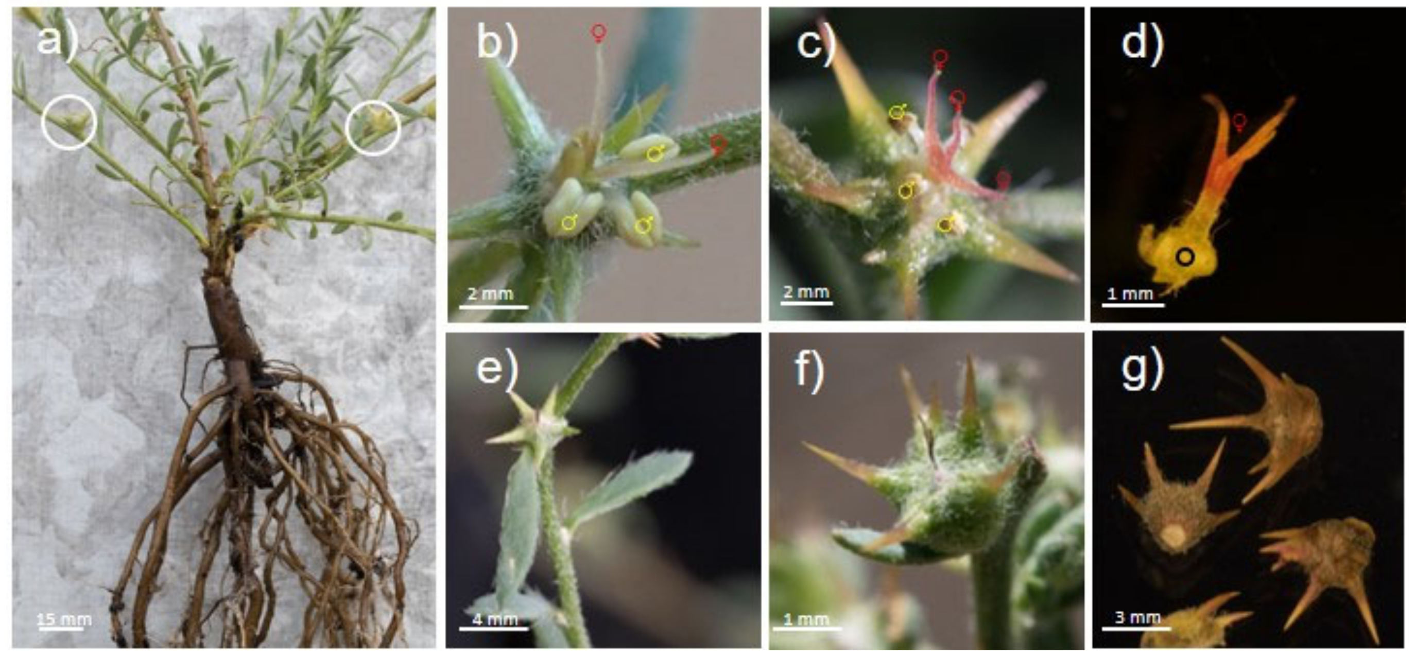
2.1. The Study Species
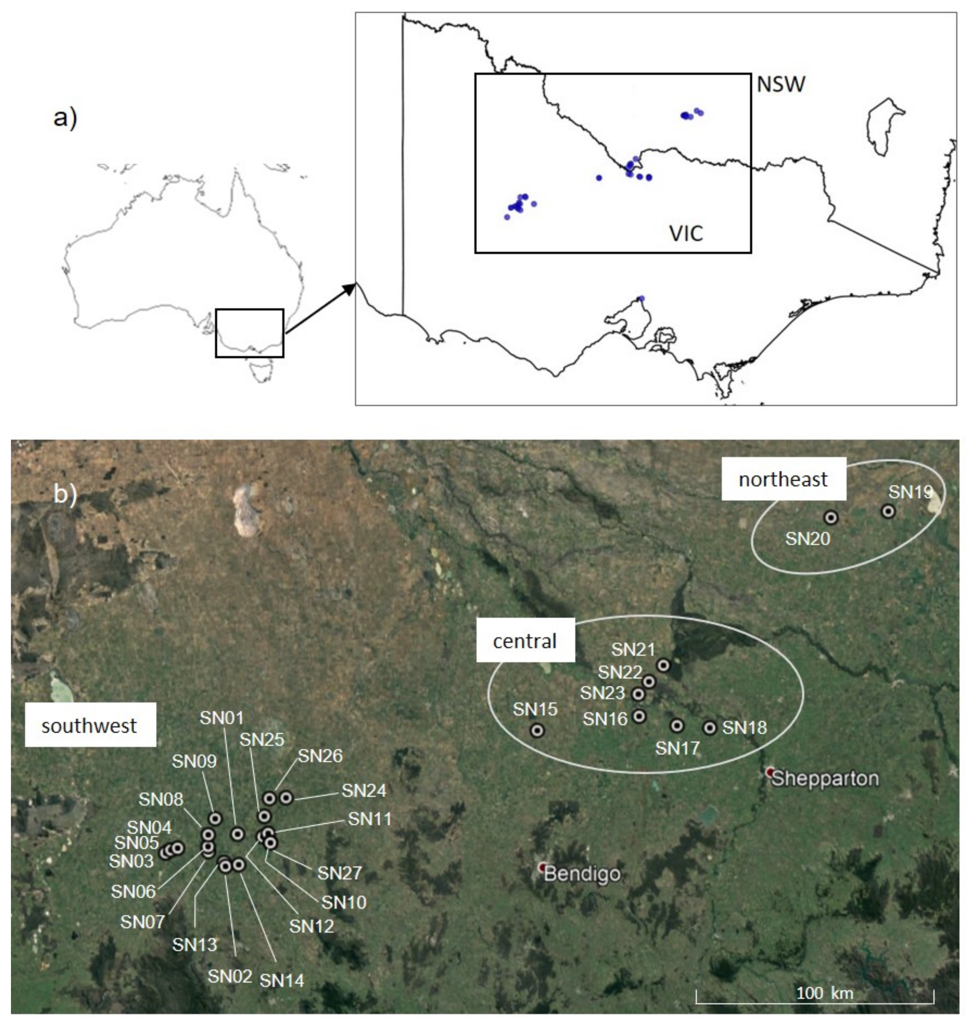
Sclerolaena napiformis is restricted to three disjunct regions in the semi-arid Murray Darling Depression and Riverina regions of Victoria (Vic) and New South Wales (NSW) in southeast Australia. We designated the following regions: “northeast” (NSW only), where only two populations were found; “central”, with populations north and south of the Murray River; and “southwest” (Victoria only), containing the greatest number and density of populations (Figure 1). The species grows as a procumbent multi-stemmed, perennial sub-shrub up to 40 cm high, mainly in native grassland and remnant Buloke (Allocasuarina luehmannii) woodland habitats. A thick rootstock develops within one year of germination and plants can re-shoot from the stem base following dieback in response to environmental conditions [23]. The floral morphology of S. napiformis is typical of wind pollination, and the fruiting perianth, a burr, has spines, suggesting dispersal by animals (zoochory) (Figure 2). The breeding system has not been studied but seed is produced if plants are bagged to exclude pollen from a different individual; thus, we assume S. napiformis to be self-compatible (James, unpublished data), as apomixis has not been recorded in the genus. At a few sites, the species commonly associated with at least low levels of salinity are present (e.g., Atriplex semibaccata, Salsola tragus subsp. tragus, Spergularia brevifolia), but overall, the associated vegetation carries little signal of salinity. All collection sites comprised primarily native species where weeds may have been present but did not dominate the site, suggesting that S. napiformis is not tolerant of significant modification of the original vegetation.

2.2. Sampling

For population analysis (ddRADseq and chloroplast haplotying), we visited 44 sites from February to April in 2018 (late summer to mid-autumn) following identification of sites using location information taken from herbarium specimens in the Australasian Virtual Herbarium (avh.ala.org.au) and observation records in the Atlas of Living Australia (ala.org.au). No plants were found at 15 sites and populations at two sites had insufficient leaf tissue to sample. The 27 sites sampled across the species’ geographic range varied in area from 0.06 to 1.25 ha and contained discrete (sub)populations varying in size from approximately 40 to 400 individuals. Plants were sometimes cryptic, and thus these estimates, which were based on observed plants, were generally conservative. Sampled plants were geolocated and fresh leaf material was collected from 9–22 mature plants per population and desiccated in silica gel (Figure 1, Table 1).
In addition, two samples, grown from seed collected from Trevaskis Rd (SN18, central region) and South Corree Rd (SN20, northeast region), were used for whole genome Illumina shotgun sequencing to provide a genome scaffold for ddRADseq SNP loci. Chloroplast reference genomes [38] were assembled from the same sequence data and used for haplotyping.

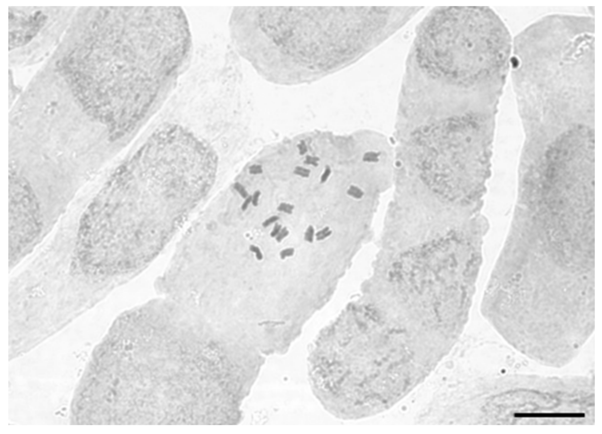
2.3. Chromosome Counts

To assist in the analysis of ddRADseq data, we determined the ploidy of S. napiformis by chromosome counts. Actively growing root tips were collected from ex situ plants grown from seed collected at populations SN12, SN18, SN20 (at or very near the site of the type collection), and SN24. Root tips were prepared using a modification of the method of Murray and Young [39] by pre-treatment in a saturated 1,4-dichlorobenzene solution at 20 °C for 24 h, then fixation in 3:1 95% ethanol/glacial acetic acid at 4 °C for 24 h. Root tips were rinsed several times in water and either stored in 70% ethanol at −20 °C or prepared immediately for counts by hydrolysing root tips in 10% HCl for 8 min at 60 °C, macerated in a drop of FLP orcein stain [40], then squashed and viewed under oil immersion. Chromosome counts were made from cells across several root tips per plant.

2.4. DNA Isolation and Sequencing

Leaf material was dried to maximise DNA preservation during extensive field surveys. Dried leaf material (≈20 mg) was ground to a fine powder in a QIAGEN TissueLyser II (two minutes) and genomic DNA was isolated using the CTAB protocol for ISOLATE II Plant DNA Kit (Bioline)—except that final elution was in a total volume of 40 µL elution buffer. DNA quality was confirmed via 1% agarose gel electrophoresis in 1xTBE buffer for 45 min at 100 V and stained with SybrSafe (Invitrogen, Thermo Fisher Scientific Australia). DNA isolations were quantified using a Qubit v3.0 fluorometer (Invitrogen Life Technologies) and stored at −20 °C.

2.4.1. Whole Genome Sequencing

To improve identification of loci from the ddRADseq reads, we obtained a de novo reference scaffold using Illumina shotgun sequences. Genomic DNA (CTAB protocol for ISOLATE II Plant DNA Kit; Bioline Australia) was isolated separately from fresh leaf material sampled and vouchered from 2 cultivated plants grown using seed sourced from Jerilderie, New South Wales (MEL2470835A) and near Wyuna, Victoria (MEL2446779A). A genome library was prepared for each sample using a TruSeq Nano DNA Library Prep kit (Illumina, San Diego, USA). A minimum of 2.5 µg genomic DNA template of each sample was supplied to Australian Genome Research Facility (AGRF; Parkville, Aust) at 50 ng/µL and sequenced (150 bp PE on an Illumina NovaSeq 6000).

2.4.2. ddRADseq

A modified version of the Peterson et al. ddRADseq protocol [37] was used to prepare DNA libraries—details are available at michaelamor.com/protocols. The final DNA library contained 480 samples, which included 13 technical replicate pairs. Individuals were randomly allocated to a plate per well and therefore received a random barcode and index. In summary, 100 ng of genomic DNA was digested for 18 h with EcoRI-HF and AseI restriction enzymes (New England Biolabs) and barcoded adapters were ligated to digested DNA fragments. Non-ligated adapters were removed before libraries were size-selected by magnetic bead purification using Jetseq Clean (Bioline)/PEG 8000 buffer solution at 0.5× then 0.9× of the DNA solution volume.
PCR-based indexing of the individual libraries was conducted using real-time PCR (rtPCR) in a Bio-Rad CFX96 thermocycler, with amplification stopped after 10 cycles. To assess whether amplification was adequate for sequencing whilst minimising PCR bias, we visualised individual fluorescence curves to ensure that they had not plateaued. Amplified libraries were pooled in equal concentrations based on relative fluorescence unit outputs from rtPCR and were concentrated/purified using Jetseq Clean beads/PEG 8000 buffer solution (1.8× DNA solution volume). The pooled library was size-selected at 300–500 bp in a Pippin Prep (Sage Science) using a 2% agarose (100–600 bp) cassette and quantified via qPCR using a Jetseq Library Quantification Hi-ROX kit (Bioline) on a Bio-Rad CFX96 thermocycler. Library QC and sequencing were performed at the AGRF.

2.5. Quality Filtering and Bioinformatics

2.5.1. Nuclear DNA Assembly

Genome scaffolds for each sample were assembled as follows. Quality filtering of reads was performed using Trimmomatic 0.39 [41] with the following settings: LEADING:3 TRAILING:3 SLIDINGWINDOW:4:20 MINLEN:36. Paired reads were then normalised to ≈100× coverage using BBnorm (settings: mindepth = 5 target = 100). Normalised reads were assembled into scaffolds using SPAdes v3.13.0 [42]. Benchmarking Universal Single-Copy Orthologs (BUSCO v3.1.0; [43]) statistics were applied to assess the completeness of the assembly. To estimate the recovery of gene-coding regions in the resulting assembly, we assessed scaffolds with BUSCO using the embryophyta_odb10 database (settings: -m genome -sp arabidopsis).

2.5.2. Population Samples (ddRADseq)

Raw paired-end reads were trimmed if the quality dropped below a score of phred20, based on a sliding-window of four bases using Trimmomatic v0.38 [41]. Reads below our minimum length requirement of 100 bases were discarded. Finally, reads were trimmed if Illumina adapters were present and filtered for microbial and fungal contaminants using Kraken v2.0.6 [44]. Reads were demultiplexed into individual sample read sets using the “process_radtags” feature of STACKS v1.4.6 [45].
Assembly of reads into loci was performed on (i) reads 1 and 2, and (ii) only read 1 using ipyrad v0.7.29 [46]. Reads were assembled using a stepwise approach by mapping reads to our most reliable genome scaffold (determined by size (gb) and BUSCO score) and performing de novo assembly on the remaining reads. Inclusion of read 1 only resulted in more loci in all cases, and therefore assemblies based only on read 1 were used downstream. Further sequence quality filtering was performed to convert base calls with a score of <30 into Ns, whilst excluding reads with ≥15 Ns. Our complete assemblies required minimum depth of 10x reads per locus. The resulting assemblies were used to generate variant call format (VCF) files for population genomic analyses and alignment (phylip) files for chloroplast (cp) DNA-based haplotyping.
The occurrence of outlier loci, interpreted as candidates for loci under selection, was assessed for all assemblies using Bayescan v2.1 [47] and a Principal Component Analysis (PCA) approach implemented via the “pcadapt” package [48] in R 3.5.3 [49]. Only sites identified by both methods were considered true outliers. BayeScan (10,000 pilot runs and 200,000 generations, with 50,000 initial generations discarded as burn-in) identified zero outliers compared to 104 outliers detected by “pcadapt”. As no outliers were common across both approaches, we considered those identified by “pcadapt” to be false positives, and the following analyses were conducted using all loci.

2.5.3. Population Samples (cp Haplotyping)

Reads from the ddRADseq libraries were mapped to a consensus sequence of two S. napiformis individuals (GenBank Accessions MT027236 and MT027237 [38]) using ipyrad [46]. The clustering similarity threshold was set to a minimum of 80% and the presence of ≥50 individuals per locus. An alignment including the two reference genomes was visualised in Geneious Prime v2020.1.2 (https://www.geneious.com). A summary table of variable sites was created manually, and a haplotype network was constructed in R 3.5.3 using the “pegas” package [50].

2.6. Analysis of Genetic Diversity and Structure

Genetic structure was investigated among and within regions using a step-wise approach via the “fastStructure” algorithm [51]. VCF files generated by ipyrad were converted to ped and map files using VCFtools v0.1.15 [52], then further converted to bed, bim, and bam files using PLINK v1.90b4 [53]. To identify genetic clusters, we performed 8 to 10 replicate runs for each K-value (number of sites minus 1) based on our complete assembly using the logistic model with 10 cross-validation steps for each run. FastStructure outputs were summarised with Clustering Markov Packager Across K (CLUMPAK) “main pipeline – admixture” and “best K” algorithms via the online server (http://clumpak.tau.ac.il/). We attempted 150 fastStructure replicate runs for each K-value for our regional analysis, however, a high failure rate resulted in us retaining >10 replicates for K = 3 but only two completed replicates for both K = 2 and K = 4. Due to low (and uneven) replicate numbers, we were unable to summarise using CLUMPAK. Therefore, regional analyses were summarised using fastStructures with “chooseK.py” and “distruct.py” scripts to enable presentation of the single “best” graphical representation and its associated likelihood values. To investigate potential sub-structure between the two northeast sites, we performed fastStructure analyses using an assembly generated from individuals from the northeast and central sites. We compared the Bayesian-based genetic clusters obtained from fastStructure with those identified using K-means clustering and Bayesian information criterion (BIC) as implemented for discriminant analysis of principal components (DAPC [54]). To support the above findings, we investigated correlation between genetic and geographic distance using Mantel’s R statistic via the “mantel” function in the “vegan” R package [55]. Geographic (Euclidean) and genetic distance (dissimilarity) matrices were calculated with the “dist” and “bitwise.dist” functions in R, respectively, using the package “poppr” [56].
For population genomic level analyses within and among regions, we imported VCF files into R and converted them to “genind” and “hierfstat” objects. Estimates of genetic differentiation were calculated via pairwise GST and Jost’s D among our identified regions using the “mmod” R package. The degree of genetic differentiation among regions was estimated via 1000 permutations of analysis of molecular variance (AMOVA) using the “poppr” R package. Euclidean genetic distance was input as a covariate using the “pegas” algorithm. Global and regional estimates of genetic diversity were calculated based on the observations resulting from our population structure analyses. We estimated observed heterozygosity (Ho) and gene diversity (He) using the “basic.stats” function in the “hierfstat” R package. Global FIS was estimated via the “boot.ppfis” function in the “hierfstat” R package [57] to determine the proportion of species-wide and region-wide genetic variation reflected in individuals. Global FST and GST was estimated via the “wc” and “Gst_Hedrick” functions in “hierfstat” and “mmod” [58], respectively.

2.7. Distribution Modelling

We investigated the potential for habitat/environment suitability to shift under a conservative climate change scenario using 20 variables (Table S1). A total of 8 soil variables (3 seconds resolution) were downloaded from the CSIRO soil and landscape database (http://www.clw.csiro.au/aclep/soilandlandscapegrid/index.html). A total of 12 bioclimatic variables (30 seconds resolution) were downloaded from the WorldClim database (www.worldclim.org/bioclim) as “current conditions” (interpolations of observed data, representative of 1960–1990) and “future conditions” (IPCC5 climate projections for 50 years assuming the most conservative “representative concentration pathway” (RCP = 2.6) for greenhouse gases). Collection coordinates were used as species occurrence data, which is the most extensive collection to date and was informed by >30 years of field surveys.
The extent of the models was set to 10 degrees surrounding occurrences (site locations). Each model was fitted using the maximum entropy (Maxent) algorithm via the dismo package in R [59]. Model fit was evaluated by simulating 1000 random pseudoabsences within the model extent and tested how well our collection data compared to “random guessing” using a receiver operating characteristic (ROC) curve (AUC = 0.994; Figure S1a). We considered this to be a realistic approach to obtaining absences, as true absence data are difficult to obtain for S. napiformis because plants can die down to ground level under stressful conditions [23]. Variable contributions were plotted for (i) current climate, (ii) soil, and (iii) current climate and soil combined (Figure S1b). We used the raster package in R [60] to predict the suitable habitat for S. napiformis in 2050 using our “future climate” variables and including soil data with the assumption that soil and landscape will remain constant.

3. Results

3.1. Chromosome Counts

All counts were consistently 2n = 18 chromosomes (Figure 3). A diploid number of 2n = 18 was reported for Sclerolaena birchii (recorded as Bassia birchii, [61]), the only other species of Sclerolaena for which chromosome numbers are available. Therefore, we considered S. napiformis diploid, and ploidy was specified as such where required for analysis.

3.2. Data assembly Statistics

Our nuclear genome assembly (built using short reads) was ≈6.5 million nucleotides in length and consisted of 733,636 contigs (average length = 888.27, largest length = 154,606). Overall, 1145 complete genes were identified (83% of the 1375 total recognised genes), 137 genes (10%) were partially identified (fragmented sequence), and 93 (6.7%) were missing.
For ddRAD data, the final analysed dataset consisted of 452 individuals. Summary statistics are provided in Table 2. After filtering loci and informative sites for each assembly, the number of unlinked SNPs ranged from 2837 to 3367 with a mean depth of ≈15 reads per individual at every retained locus. For all assemblies, approximately 31% of reads were mapped to our assembled genome scaffold.

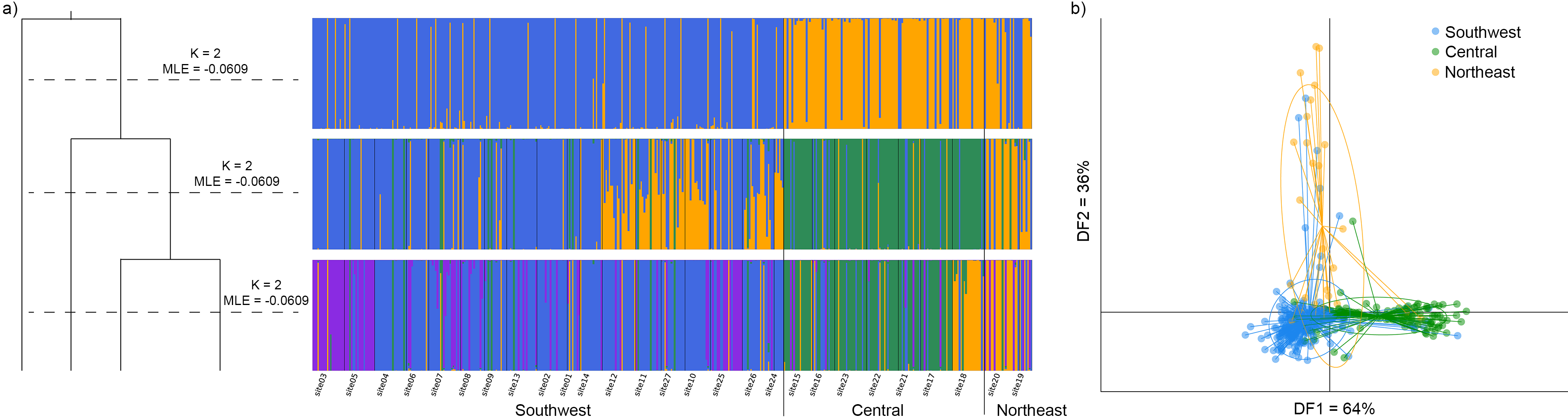
3.3. Regional Genetic Diversity and Structure

Measures of regional genetic diversity are summarised in Table 3. Genetic structure among regions was supported by AMOVA (see Tables S2–S5), where 8.7% of the total variation was observed among southwest, central, and northeast regions (p = <0.001). AMOVA also provided support for differentiation among sites within the southwest and northeast regions (p = <0.02), but not among sites within the central region (p = 0.8). Correlation between genetic and geographic distance (Mantel’s R) was significant among regions (p = 0.001), and among sites within the central region (p = 0.04). There were no noteworthy correlations among sites within the southwest or northeast region. Overall, S. napiformis was characterised by relatively low levels of heterozygosity (Ho = 0.017), with a high proportion of the overall genetic diversity captured within a given individual (FIS = 0.617), pointing to notable levels of inbreeding/selfing within the species. This trend was consistent when looking within regions where heterozygosity levels (Ho) were relatively low but diversity within individuals (FIS) was high. All sites exhibited FIS values consistent with substantial levels of selfing, except SN24, where the FIS value was negative (Table S6), suggesting clonal reproduction was greatest at this site. There was no correlation between FIS and population size, population area, or the number of samples included in the estimation of FIS.
Analyses among the three disjunct regions showed that sites within the southwest, central, and northeast all had greater gene diversity than heterozygosity and were characterised by a high degree of inbreeding/selfing (FIS = 0.517, 0.652, and 0.830, respectively). Population differentiation among sites was similar within the southwest and central regions (GST = 0.304 and 0.288, respectively) but higher for the small northeast region (GST = 0.369). Comparing pairwise genetic difference between regions, we found the central and northeast regions to be the most distinct (pairwise GST = 0.228, Jost’s D = 0.017; Table 4), despite being geographically closer than either was to the southwest.

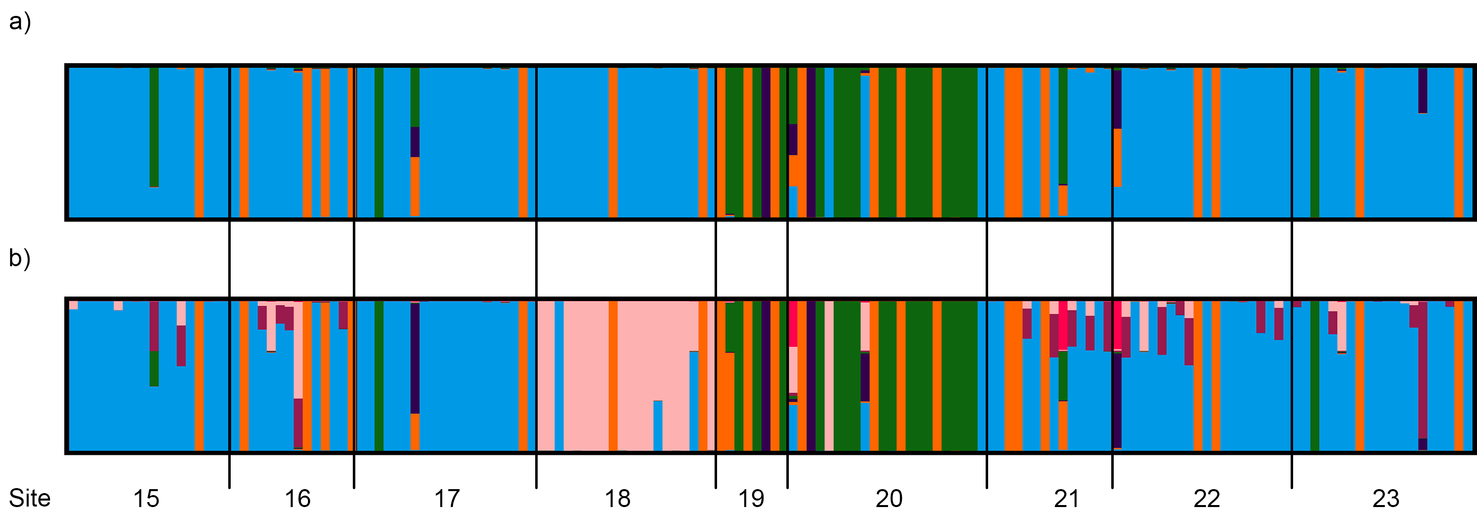
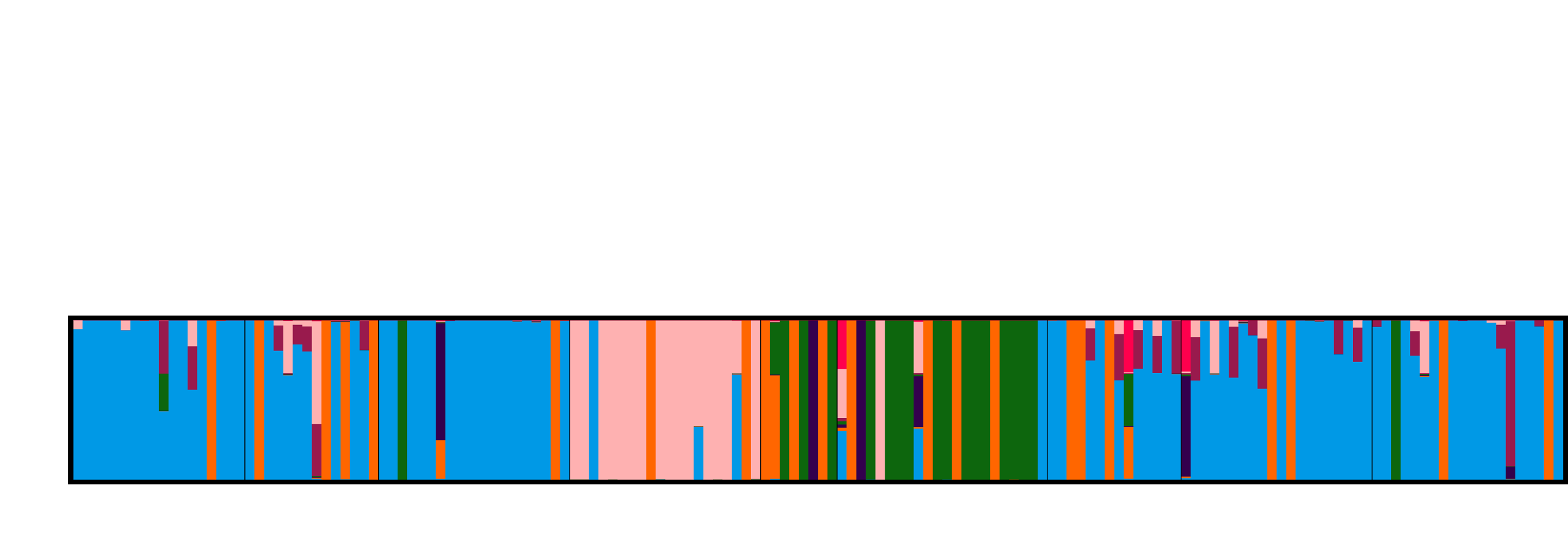
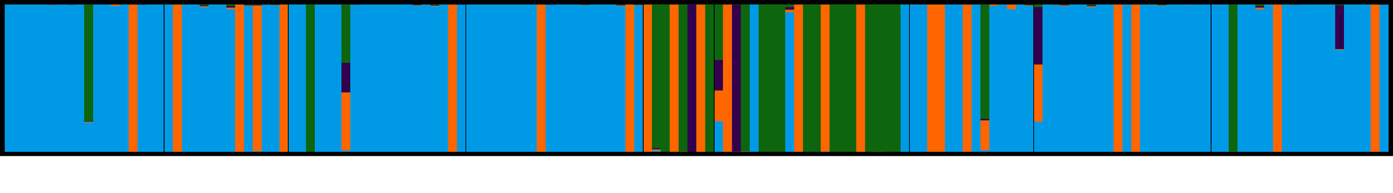
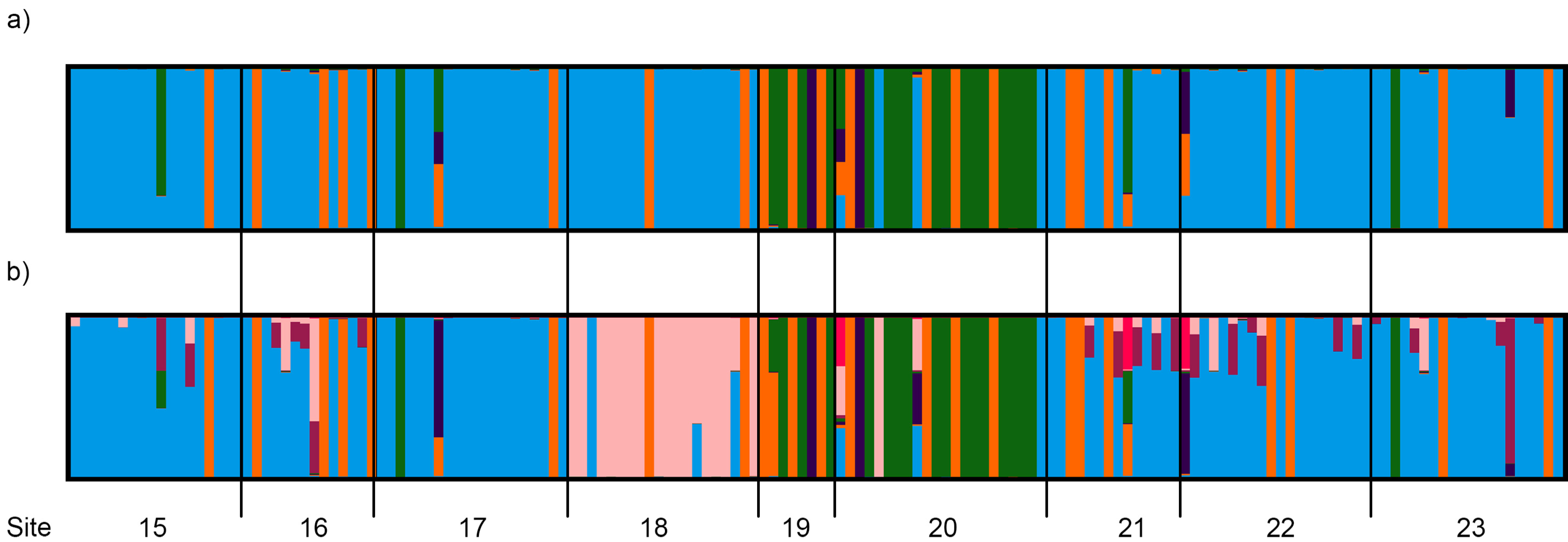
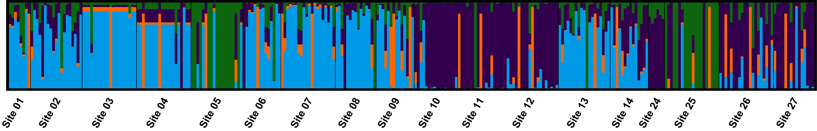
3.4. Population Genetic Structure

3.4.1. Overview of All Regions

Population structure was examined for the species across the geographic range. Marginal likelihoods resulting from fastStructure runs of the regional assembly of S. napiformis favoured four distinct genetic clusters with clear differences shown among geographic regions (Figure 4a). For K = 4, individuals assigned to blue and purple clusters were widely dispersed geographically but most common in the southwest region, whereas individuals from green and yellow clusters were mostly found in the central and northwest regions, respectively. DAPC identified the optimal number of clusters as three (Figure S2), and also showed differences among groups of individuals on the basis of their geographic region, but samples from the northeast were less tightly clustered than the majority of samples from the central and southwest regions (Figure 4b).

3.4.2. Central and Northeast Regions

For the combined central and northeast regions, the optimal number of clusters identified from both fastStructure and DAPC was K = 4, although K = 7 was also a possibility (Figure S2). The distribution of clusters was not always well correlated with geographic location. Visualising the fastStructure output (Figure 5), at K = 4, the two northeast sites (19 and 20) were delimited from other sites but could not be distinguished from each other (Figure 5a). At K = 7, three groups were evident, with site 18 (central) and sites 19 and 20 (northeast) distinct from all other sites, which were dominated by a single genetic cluster (blue—Figure 5b). The remaining 1–4 clusters (K4 vs K7) were made up by very few individuals dispersed seemingly randomly across localities. DAPC was less successful at delimiting sites within the combined central and northeast region (Figure S3).

3.4.3. Southwest Region

The optimal number of clusters within the southwest region as identified by fastStructure was K = 4 (Figure 6), with populations showing variable levels of admixture. There was a loose geographic association with the more westerly sites being mainly cluster 1 (blue) and more easterly sites (10, 11, 12, 24, 26, and 27) being mainly cluster 2 (purple). Sites 5 and 25 had high membership probability to cluster 3 (green) that was not explained by habitat or proximity. Cluster 4 (orange) showed no geographic association. Although not definitive, DAPC suggested six genetic clusters as the lowest likely value of K and no substantial geographic structure with most individuals assigned to a single widespread genetic cluster (Figure S4).

3.5. Chloroplast Genomes and Haplotyping

We obtained 17 loci comprising 7 informative sites by mapping the ddRADseq reads to two chloroplast reference genomes (GenBank accessions MT027236 and MT027237). None of the informative sites mapped to the most variable chloroplast regions identified in the alignment of the reference genomes. Two informative sites corresponded to partial sequences of the matK gene, a variable site when comparing GenBank sequences for other species of Sclerolaena. The remaining informative sites did not correspond to any chloroplast sequences available for Sclerolaena. Although eight haplotypes were recognised, only six were differentiated if variable positions containing “N” were ignored, and while 59% of populations had more than one haplotype, it was not possible to identify relationships to sites or regions (Table 5). The star-shaped haplotype network (Figure S5a) is consistent with a single maternal lineage dominated by one haplotype, H1, and a few minor variants derived by mutation [62,63]. Haplotype H1, possibly ancestral, dominated overall and was recovered from 351/390 individuals spread across the 27 sites. The second most common haplotype, H2 (21/390 individuals), was found at 10/27 sites (37%) and in most individuals (9/14) at site 25, the only site where H1 was not the most common haplotype (Figure S5b).

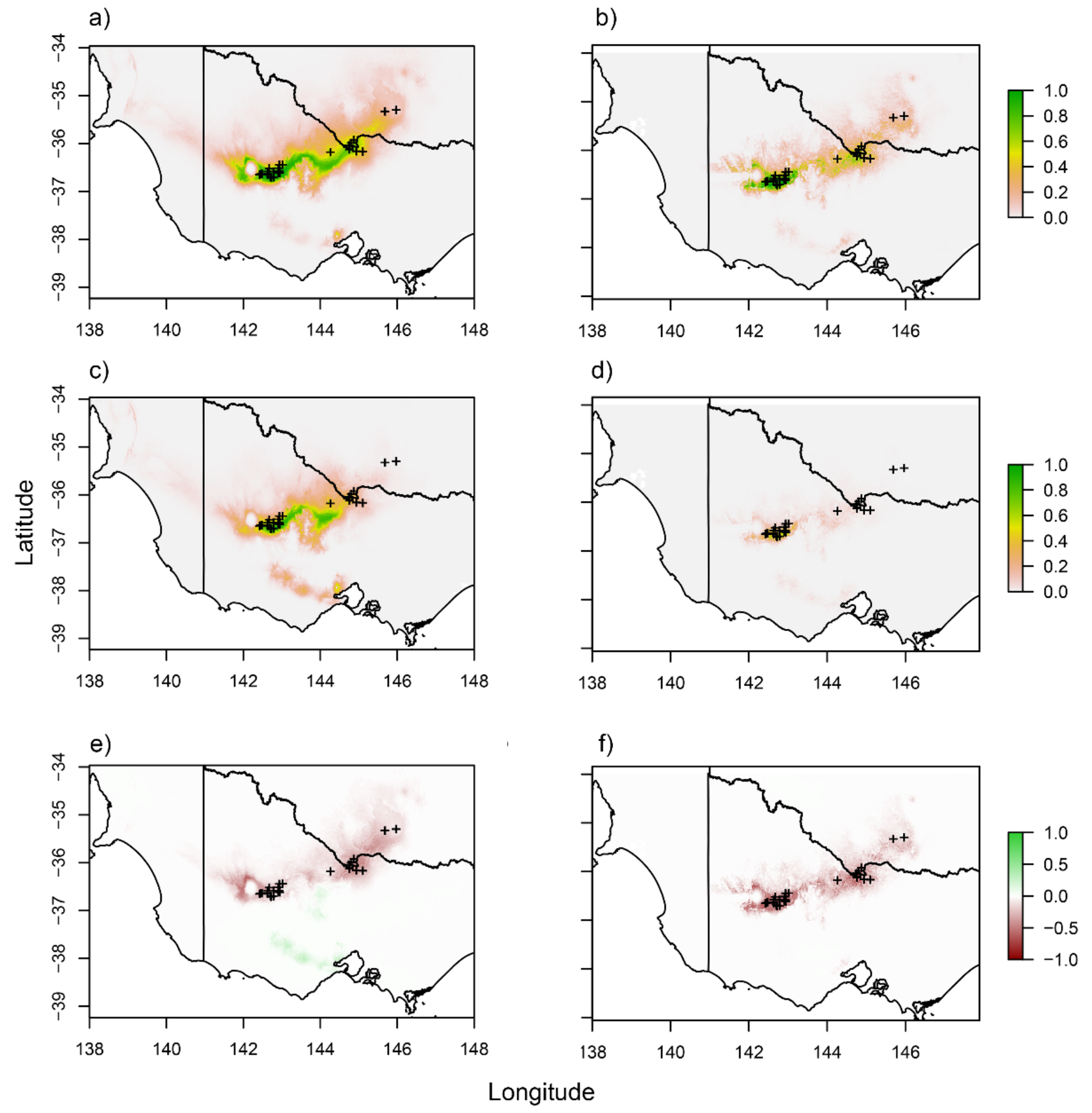
3.6. Distribution Modelling

Investigating the variables most associated with the occurrence of S. napiformis revealed that most variation in the model was accounted for by the presence of clay in the soil (≈50%) and the annual mean temperature (≈15%). Carbon and other climate variables associated with precipitation and temperature all contributed >5% towards the total observed variation (Figure S1b). Overall, a decrease in available suitable environment was predicted for the next 50 years using both models: climate variables only and a combination of climate and soil variables. Combining soil types with climate variables decreased predicted present and future suitable environment substantially when compared to the climate-only model. Additionally, the climate-only model highlighted a more southerly area that increased in suitability at approximately −38 degrees latitude. Including soil type almost entirely excluded this area, as the presence of clay soils played a major role in predicting present day occurrences (Figure 7).

4. Discussion

We provide evidence for genetic structure among three disjunct regions of S. napiformis in southeast Australia. We did not find genetic differentiation among sites within central and northeast regions, but clear genetic structure was evident in the southwest region (east and west of Marnoo, Victoria). Our findings of regional differentiation of S. napiformis are consistent with limited long-distance dispersal (likely impacted by range disjunction), but also point to some historical dispersal beyond extant populations. Lower than expected heterozygosity, as well as high FIS values, also indicates substantial inbreeding within populations of S. napiformis, a self-compatible, wind-pollinated species. Effective gene-flow is unlikely to be maintained across the distribution of this species, particularly given that human-mediated landscape changes have created barriers to gene-flow and access to suitable habitat. Even if pollen-mediated gene-flow is maintained among existing sites, the probability of new sites being colonised is low without human intervention. Importantly, we did not find geographically correlated cryptic lineages of S. napiformis, in contrast to findings for other disjunct species (e.g., [26]). We suggest that conservation management of S. napiformis utilises the genetic diversity found in all populations from the northeast, central, and southwest (divided into east and west sites) to maximise the adaptability of the species in increasingly novel environments.
We also show that the current distribution of S. napiformis is restricted by soil type and tightly linked to temperature and precipitation. As such, climate projections suggest that over half the existing habitat will become unsuitable for S. napiformis over the next 50 years. Whilst we predict a decline in habitat suitability across the entire species distribution, our projections suggest that populations in the southwest region are the most likely to persist under future climate projections. Overall, our findings highlight the complexities of managing the competing demands of human utilisation and conservation of native species in the face of climate change, but we outline some viable options below.

4.1. Fragmentation, Genetic Structure, and Gene-Flow

We recorded a single dominant cpDNA haplotype across the distribution of S. napiformis, which is consistent with historical broad-scale seed dispersal, although low coverage obtained via our non-cpDNA targeted approach may limit our ability to distinguish finer-scale patterns [64]. Our findings based on nuclear DNA show clear genetic differentiation among regions and highlight finer-scale structure in the southwest region. Therefore, dispersal in S. napiformis appears most common at relatively small scales (i.e., within 20–80 km), despite seeds having morphological adaptations that promote long-distance dispersal by birds and mammals. Relatively localised dispersal is considered common among plants [65,66], although genetic studies confirming this assumption are lacking [67]. Here, we provide valuable genetic evidence that seed dispersal does not maintain genetic homogeneity over the entire (≈370 km) linear range of S. napiformis.
Human activity (land clearing and fragmentation) has reduced suitable/available grassland habitat in this area by as much as 99% [23], which has clearly contributed to the isolation of extant populations and sites. However, we identified two genetic clusters in the southwest region, which were separated by ≈11 kms and displayed no obvious landscape barrier. As many of our sites are isolated by greater distances, we believe proximity alone cannot account for reduced connectivity among S. napiformis populations, despite extreme alteration to the landscape. Similarly, a sympatric species, Pimelea spinescens, was considered to have genetic structure that pre-dated fragmentation resulting from agriculture post-colonisation [68], as also observed in other plant systems [69,70]. We therefore suggest that the genetic structure observed in S. napiformis (northeast, central, and southwest—east and west division) was present prior to colonisation, although recent land conversion will likely have downstream consequences on genetic patterns.
Certainly, habitat loss and fragmentation displace biodiversity and biomass, and this is particularly problematic for grassland systems [71]. There is no doubt that the extreme alteration to the landscape has displaced organisms that historically assisted dispersal in S. napiformis. For example, the endangered plains-wanderer Pedionomus torquatus consumes the seed and leaves of Sclerolaena spp. [72]. Despite a small home range of 7–21 ha, this bird may have historically assisted in seed dispersal among sites when both P. torquatus and S. napiformis were more common. Ants also assist in the short-distance dispersal of a closely related (and sometimes co-occurring) species, Sclerolaena diacantha [73,74], although this has not been shown explicitly for S. napiformis. Furthermore, vehicles and grazing stock may contribute to the dispersal of this common “roadside” species, although we believe these roadside populations are more likely to reflect the remaining suitable habitat for this species.

4.2. Genetic Diversity and Inbreeding

We observed high levels of inbreeding and homozygosity in discrete S. napiformis regions (and 26/27 sites), which suggests a high degree of self-pollination. Indeed, a closely related species, S. diacantha, has an estimated selfing rate of 70% with strong selection for outcrossed progeny considered unlikely [73]. Sclerolaena napiformis may display similar selfing rates to S. diacantha, given that these species largely co-occur and thus experience similar environmental pressures. Mixed mating systems, whereby plants undergo both selfing and outcrossing, can minimise the accumulation of deleterious alleles [75], even following inbreeding depression [76] or under novel or changing environments [77]. This mechanism may be used by S. napiformis as a short-term counterbalance to the negative fitness consequences associated with selfing. It may also enable recruitment into new sites from a single or few related individual/s [13,69]. For example, the inbreeding species Geum urbanum showed high levels of homozygosity and selfing without any negative consequences for fitness [78]. We note, however, that negative genetic consequences associated with a reduced gene pool may still develop over a longer timeframe [13] and, considering the extreme habitat degradation in this system and the potential establishment of populations from few individuals, we believe there is a strong requirement for further genetic monitoring of S. napiformis.

4.3. Considerations for Persistence of S. napiformis

Our modelling suggests that climate change will substantially decrease the suitability of remaining habitat for S. napiformis, even under the most conservative projections. As the climate warms, organisms are required to adapt and/or shift their distribution to track suitable climate envelopes [79]. However, most plants are unlikely to migrate fast enough to keep pace with the current rate of climate change [17]. Furthermore, the reliance of S. napiformis on clay soil compounds this, as suitable soil is rare outside of its current distribution. We therefore believe it is unlikely for S. napiformis to undergo a range-shift naturally, leaving it exposed to increasingly unsuitable environmental conditions. Furthermore, climate change is predicted to favour an increase in weediness, particularly within an agricultural setting [80]. We expect this to further reduce habitat quality for S. napiformis as competition with invasive species increases. Therefore, we consider the persistence of S. napiformis into the future unlikely without human intervention, even if an effort is made to ensure remnant patches are protected. Active restoration and rehabilitation of converted land would thus go a long way towards ensuring the persistence of S. napiformis and the grasslands of southeast Australia.
The seeds of S. napiformis tolerate a wide range of temperatures, similar to other congeneric taxa (e.g., Sclerolaena bicornis [81] and S. birchii [61]). They are produced in high volume; may remain viable while dormant for several years [82,83]; and germinate rapidly once the physical barrier of the persistent, woody perianth is removed [81,84]. Furthermore, germination of S. napiformis seed is linked to sufficient rainfall and removal of the perianth, rather than being tied to a specific time of year [61,85]. This strategy of “germinating rapidly when most advantageous” may be favourable when rainfall is erratic, and might explain why S. napiformis alters its phenology to avoid water stress at sensitive stages of its life cycle [35]. Sclerolaena napiformis also appears to flower and reproduce year-round, and again, this is partly determined by the availability of water (personal observation). This finding, and the above-mentioned germination triggers, support the notion that water availability, rather than temperature, may have a greater influence on S. napiformis establishment and successful persistence upon encountering a new site. For example, drought sensitivity is known to limit plant distribution and recruitment, particularly if it impacts early-life stages [86]. Recruitment into new areas is likely to be more restricted than germination because of the additional sensitivity during seedling establishment; however, the volume of seeds contained in the natural soil seedbank allows for mass germination when conditions are suitable [84,87]. This greatly increases the likelihood of establishing a viable population in a new area once a small number of recruits reach maturity.
Finally, we observed that the northeast region contained the lowest number and poorest quality of mature plants in terms of plant size and seed production. However, we observed good survival and healthy growth of northeast seedlings cultivated under optimal ex situ conditions. Throughout the distribution of S. napiformis, reduced available habitat, altered fire regimes, hotter/drier conditions with decreasing precipitation, and increased biomass of weeds threaten populations with local extinctions. This is particularly likely in the northeast region, and therefore retention of the genetic diversity in this area is particularly important as plants here may harbour adaptations to the predicted future conditions for central and southwest regions. We believe all populations of S. napiformis will require assisted restoration in the future, and therefore consider seed-banking from each region (particularly the northeast) a conservation priority.

5. Conclusions and Implications for Conservation

For S. napiformis to persist, conservation efforts must balance the rate of local extinction (measured as population loss) with the colonisation of new sites. Successful conservation will rely partly on management strategies that facilitate connectivity among S. napiformis sites and consider the projected effect of climate change when identifying candidate localities. High fecundity of mature plants and long-term storage capacity of germplasm will benefit conservation, and even though the development of an ex situ seedbank is underway, continued collections from diverse populations over multiple time periods is recommended.
Small populations are more vulnerable if their genetics and evolutionary biology are not integrated into the conservation strategy [88]. Although most remaining populations of S. napiformis have <200 individuals, they also have an unusually high proportion of reproductive plants [2], which lessens the risk of diversity loss in translocated or artificial populations [89]. Both inbreeding and outbreeding depression are potential risk factors when combining germplasm or augmenting gene-flow [32,88]. Outbreeding depression is considered to be less of a risk [31,32] as it is most likely when combining lineages with greater genetic distinction than we observed here [32]. We consider the greatest risk for S. napiformis to be associated with losing overall genetic variation if entire sites/regions are extirpated [27].
On the basis of our observation of sub-optimal gene-flow, we recommend the establishment of intermediate sites, with a particular focus on the southwest region, which we identified as the most likely to persist beyond our 50-year projection. As introduction/translocation only impacts genetic structure or adaptation when migrants establish and reproduce, the choice of recipient sites and ongoing monitoring is crucial to maximise the long-term success of any conservation efforts. Patterns of genetic diversity are not necessarily related to adaptive traits; therefore, quantitative approaches are likely to improve conservation success (see [6,7]).
Wide road verges (including some travelling stock routes (TSR) in New South Wales) often consist of high-quality native grassland/open woodland vegetation and some contain remnant S. napiformis populations. Roadside areas where S. napiformis is currently absent should be considered as candidate sites for establishment of corridors to facilitate gene-flow, ideally comprising plants with mixed genetics from each of the three regions. The provision of dispersal corridors by maximising the use of substantial TSRs and road verges in the area is a feasible and cost-effective conservation action. However, we believe the most beneficial conservation measure would be to open converted land for restoration of native grasslands, which would have wider benefits for the entire southeast Australian grassland system and the organisms that rely on it.

Supplementary Materials

The following are available online at https://www.mdpi.com/1424-2818/12/11/417/s1, Figure S1: All regions. DAPC: Bayesian information criterion (BIC) and assignments; fastStructure: DeltaK/ProbK. Figure S2: Central + northeast. DAPC: BIC, DAPC plot, assignments; fastStructure: DeltaK/ProbK. Figure S3: Southwest. DAPC: BIC, DAPC plot, assignments; fastStructure: DeltaK/ProbK. Figure S4: Haplotype network and geographic distribution of haplotypes based on mapping of ddRADseq loci to chloroplast reference genomes. Figure S5: Percentage contributions of soil and climate variables when modelling the distribution of e on the basis of occurrence data. Table S1: List of variables used for modelling suitable habitat for Sclerolaena napiformis. Table S2: Analysis of molecular variance among disjunct southwest, central, and northeast regions of Sclerolaena napiformis. Table S3: Analysis of molecular variance among southwestern Sclerolaena napiformis sites. Table S4: Analysis of molecular variance among central Sclerolaena napiformis sites. Analysis includes investigations of variance (a) between Victoria and New South Wales (states are divided by the Murray River), and (b) among all sites without consideration of state variable. Table S5: Analysis of molecular variance among northeast Sclerolaena napiformis sites. Table S6: Lower, mean and upper FIS estimates for each collection site of Sclerolaena napiformis.

Author Contributions

Conceptualisation, M.D.A., E.A.J. and N.G.W.; methodology, M.D.A., E.A.J., and N.G.W.; formal analysis, M.D.A.; investigation, M.D.A., E.A.J., and N.G.W.; resources, E.A.J. and N.G.W.; data curation, N.G.W. and M.D.A.; writing—original draft preparation, M.D.A. and E.A.J.; writing—review and editing, M.D.A., E.A.J., and N.G.W.; visualisation, M.D.A. and E.J.; supervision, E.A.J.; project administration, E.A.J.; funding acquisition, E.A.J. and N.G.W. All authors have read and agreed to the published version of the manuscript.

Funding

This research was funded by Department of the Environment and Energy, Australian Government, grant number TSRF-161 and the Royal Botanic Gardens Victoria (RBGV). The article processing charge was funded by the RBGV.

Acknowledgments

Gareth Holmes (RBGV) for preparing DNA libraries for genome sequencing; Chris Jackson (RBGV) for advice and assistance with data handling; Mirinda Thorpe, Iestyn Hosking, and Karly Learmonth (Victorian Department of Environment Land Water and Planning) for locality information, landholders, and local stakeholders who provided information, transport, and arranged access to sites; David Hines and Deanna Marshall (Trust for Nature) for incorporating plants from our collection into conservation plantings on private landholdings on the Patho Plains; and Hayley Cameron (Monash University) for valuable input into an earlier version of the manuscript.

Conflicts of Interest

The authors declare no conflict of interest. The funders had no role in the design of the study; in the collection, analyses, or interpretation of data; in the writing of the manuscript; or in the decision to publish the results.

Data Accessibility

Raw sequence data, assemblies and associated scripts can be accessed via Mendeley data (http://dx.doi.org/10.17632/664sh75jgz.1).

References

  1. International Union for Conservation of Nature (IUCN). The IUCN Red List of Threatened Species. 2020. Available online: https://www.iucnredlist.org (accessed on 21 May 2020).
  2. Garner, B.A.; Hoban, S.; Luikart, G. IUCN red list and the value of integrating genetics. Conserv. Genet. 2020, 21, 795–801. [Google Scholar] [CrossRef]
  3. McGuigan, K.; Sgrò, C.M. Evolutionary consequences of cryptic genetic variation. Trends Ecol. Evol. 2009, 24, 305–311. [Google Scholar] [CrossRef] [PubMed]
  4. Sgrò, C.M.; Lowe, A.J.; Hoffmann, A.A. Building evolutionary resilience for conserving biodiversity under climate change. Evol. Appl. 2011, 4, 326–337. [Google Scholar] [CrossRef] [PubMed]
  5. Hoffmann, A.; Griffin, P.; Dillon, S.; Catullo, R.; Rane, R.; Byrne, M.; Jordan, R.; Oakeshott, J.; Weeks, A.; Joseph, L.; et al. A framework for incorporating evolutionary genomics into biodiversity conservation and management. Clim. Chang. Responses 2015, 2, 1–23. [Google Scholar] [CrossRef] [Green Version]
  6. Reed, D.H.; Frankham, R. Correlation between fitness and genetic diversity. Conserv. Biol. 2003, 17, 230–237. [Google Scholar] [CrossRef]
  7. Kramer, A.T.; Havens, K. Plant conservation genetics in a changing world. Trends Plant Sci. 2009, 14, 599–607. [Google Scholar] [CrossRef] [PubMed]
  8. Ouborg, N.J.; Vergeer, P.; Mix, C. The rough edges of the conservation genetics paradigm for plants. J. Ecol. 2006, 94, 1233–1248. [Google Scholar] [CrossRef]
  9. Dunlop, M.; Hilbert, D.; Ferrier, S.; House, A.; Liedloff, A.; Prober, S.M.; Smyth, A.; Martin, T.G.; Harwood, T.; Williams, K.J.; et al. A report prepared for the Department of Sustainability, Environment, Water, Population and Communities and the Department of Climate Change and Energy Efficiency. In The Implications of Climate Change for Biodiversity Conservation and the National Reserve System: Final Synthesis; CSIRO Climate Adaptation Flagship: Canberra, Australia, 2012. [Google Scholar]
  10. Mable, B.K. Conservation of adaptive potential and functional diversity: Integrating old and new approaches. Conserv. Genet. 2019, 20, 89–100. [Google Scholar] [CrossRef] [Green Version]
  11. Pina-Martins, F.; Baptista, J.; Pappas, G., Jr.; Paulo, O.S. New insights into adaptation and population structure of cork oak using genotyping by sequencing. Glob. Chang. Biol. 2019, 25, 337–350. [Google Scholar] [CrossRef]
  12. Willi, Y.; Hoffmann, A.A. Demographic factors and genetic variation influence population persistence under environmental change. J. Evol. Biol. 2009, 22, 124–133. [Google Scholar] [CrossRef]
  13. Mimura, M.; Yahara, T.; Faith, D.P.; Vazquez-Dominguez, E.; Colautti, R.I.; Araki, H.; Javadi, F.; Nunez-Farfan, J.; Mori, A.S.; Zhou, S.; et al. Understanding and monitoring the consequences of human impacts on intraspecific variation. Evol. Appl. 2017, 10, 121–139. [Google Scholar] [CrossRef] [PubMed]
  14. Willi, Y.; Van Buskirk, J.; Hoffmann, A.A. Limits to the adaptive potential of small populations. Annu. Rev. Ecol. Evol. Syst. 2006, 37, 433–458. [Google Scholar] [CrossRef]
  15. Vilas, A.; Perez-Figueroa, A.; Quesada, H.; Caballero, A. Allelic diversity for neutral markers retains a higher adaptive potential for quantitative traits than expected heterozygosity. Mol. Ecol. 2015, 24, 4419–4432. [Google Scholar] [CrossRef] [PubMed]
  16. Hoffmann, A.A.; Sgrò, C.M. Climate change and evolutionary adaptation. Nature 2011, 470, 479–485. [Google Scholar] [CrossRef] [PubMed]
  17. Cunze, S.; Heydel, F.; Tackenberg, O. Are plant species able to keep pace with the rapidly changing climate. PLoS ONE 2013, 8, e67909. [Google Scholar] [CrossRef]
  18. Vitt, P.; Havens, K.; Kramer, A.T.; Sollenberger, D.; Yates, E. Assisted migration of plants: Changes in latitudes, changes in attitudes. Biol. Conserv. 2010, 143, 18–27. [Google Scholar] [CrossRef]
  19. Franklin, I.R.; Frankham, R. How large must populations be to retain evolutionary potential? Anim. Conserv. 1998, 1, 69–70. [Google Scholar] [CrossRef]
  20. Nunney, L.; Campbell, K.A. Assessing minimum viable population size–Demography meets population genetics. Trends Ecol. Evol. 1993, 8, 234–239. [Google Scholar] [CrossRef]
  21. Commonwealth of Australia. Interim Biogeographical Regionalisation of Australia, Version 7. 2020. Available online: https://www.environment.gov.au/land/nrs/science/ibra (accessed on 17 July 2020).
  22. EPBC. Environment Protection and Biodiversity Conservation Act 1999. 2016. Available online: https://www.legislation.gov.au/Details/C2016C00777 (accessed on 17 July 2020).
  23. Mavromihalis, J. National Recovery Plan for the Turnip Copperburr Sclerolaena napiformis; Victorian Government Department of Sustainability and Environment (DSE): Melbourne, Australia, 2010.
  24. Cunningham, G.M.; Mulham, W.E.; Milthorpe, P.L.; Leigh, J.H. Plants of Western New South Wales; CSIRO Publishing: Melbourne, Australia, 1992. [Google Scholar]
  25. Conn, B.J. Natural regions and vegetation of Victoria. In Flora of Victoria; Foreman, D.B., Walsh, N.G., Eds.; Inkata Press: Melbourne, Australia, 1993; Volume 1, pp. 79–158. [Google Scholar]
  26. Van Rossum, F.; Martin, H.; Le Cadre, S.; Brachi, B.; Christenhusz, M.J.M.; Touzet, P. Phylogeography of a widely distributed species reveals a cryptic assemblage of distinct genetic lineages needing separate conservation strategies. Perspect. Plant. Ecol. Evol. Syst. 2018, 35, 44–51. [Google Scholar] [CrossRef]
  27. Weeks, A.R.; Sgrò, C.M.; Young, A.G.; Frankham, R.; Mitchell, N.J.; Miller, K.A.; Byrne, M.; Coates, D.J.; Eldridge, M.D.; Sunnucks, P.; et al. Assessing the benefits and risks of translocations in changing environments: A genetic perspective. Evol. Appl. 2011, 4, 709–725. [Google Scholar] [CrossRef] [Green Version]
  28. Prober, S.M.; Byrne, M.; McLean, E.H.; Steane, D.A.; Potts, B.M.; Vaillancourt, R.E.; Stock, W.D. Climate-adjusted provenancing: A strategy for climate-resilient ecological restoration. Front. Ecol. Evol. 2015, 3, 65. [Google Scholar] [CrossRef] [Green Version]
  29. Walsh, N.G. Maireana obrienii (Chenopodiaceae), a new species from eastern Australia. Muelleria 2013, 31, 61–64. [Google Scholar]
  30. Walsh, N.G.; Sluiter, I.R.K. Lectotypification of Atriplex stipitata Benth. (Chenopodiaceae) and recognition of a new subspecies. Muelleria 2020, 38, 101–109. [Google Scholar]
  31. Frankham, R. Genetic rescue of small inbred populations: Meta-analysis reveals large and consistent benefits of gene flow. Mol. Ecol. 2015, 24, 2610–2618. [Google Scholar] [CrossRef]
  32. Frankham, R.; Ballou, J.D.; Eldridge, M.D.; Lacy, R.C.; Ralls, K.; Dudash, M.R.; Fenster, C.B. Predicting the probability of outbreeding depression. Conserv. Biol. 2011, 25, 465–475. [Google Scholar] [CrossRef]
  33. Wilson, P.G. Sclerolaena napiformis Paul G. Wilson sp. nov. Flora Aust. 1984, 4, 330. [Google Scholar]
  34. Angiosperm Phylogeny Group (APG). An update of the classification for the orders and families of flowering plants: APG IV. Bot. J. Linn. Soc. 2016, 181, 1–20. [Google Scholar] [CrossRef] [Green Version]
  35. Kadereit, G.; Newton, R.J.; Vandelook, F. Evolutionary ecology of fast seed germination—A case study in Amaranthaceae/Chenopodiaceae. Perspect. Plant. Ecol. Evol. Syst. 2017, 29, 1–11. [Google Scholar] [CrossRef]
  36. Woinarski, J.C.Z.; Braby, M.F.; Burbidge, A.A.; Coates, D.; Garnett, S.T.; Fensham, R.J.; Legge, S.M.; McKenzie, N.L.; Silcock, J.L.; Murphy, B.P. Reading the black book: The number, timing, distribution and causes of listed extinctions in Australia. Biol. Conserv. 2019, 239, 108261. [Google Scholar] [CrossRef]
  37. Peterson, B.K.; Weber, J.N.; Kay, E.H.; Fisher, H.S.; Hoekstra, H.E. Double digest RADseq: An inexpensive method for de novo SNP discovery and genotyping in model and non-model species. PLoS ONE 2012, 7, 1–11. [Google Scholar] [CrossRef] [Green Version]
  38. Amor, M.D.; Jackson, C.J.; Holmes, G.D.; James, E.A. Characterization of the complete chloroplast genome of Sclerolaena napiformis Wilson, an endangered Australian chenopod. Mitochondrial DNA B 2020, 5, 1332–1333. [Google Scholar] [CrossRef] [Green Version]
  39. Murray, B.; Young, A.G. Widespread chromosome variation in the endangered grassland forb Rutidosis leptorrhynchoides F. Muell. (Asteraceae: Gnaphalieae). Ann. Bot. 2001, 87, 83–90. [Google Scholar] [CrossRef] [Green Version]
  40. Jackson, R.C. Chromosomal evolution in Haplopappus gracilis: A centric transposition race. Evolution 1973, 27, 243–256. [Google Scholar]
  41. Bolger, A.M.; Lohse, M.; Usadel, B. Trimmomatic: A flexible trimmer for Illumina Sequence Data. Bioinformatics 2014, 30, 2114–2120. [Google Scholar] [CrossRef] [Green Version]
  42. Bankevich, A.; Nurk, S.; Antipov, D.E.A. SPAdes: A new genome assembly algorithm and its applications to single-cell sequencing. J. Comput. Biol. 2012, 19, 455–477. [Google Scholar] [CrossRef] [Green Version]
  43. Seppey, M.; Manni, M.; Zdobnov, E.M. BUSCO: Assessing genome assembly and annotation completeness. In Gene Prediction; Methods in Molecular Biology Series; Kollmar, M., Ed.; Humana: New York, NY, USA, 2019; Volume 1962, pp. 227–245. [Google Scholar]
  44. Wood, D.E.; Salzburg, S.L. Kraken: Ultrafast metagenomic sequence classification using exact alignments. Genome Biol. 2014, 1415, R46. [Google Scholar] [CrossRef] [Green Version]
  45. Catchen, J.; Hohenlohe, P.; Bassham, S.; Amores, A.; Cresko, W. Stacks: An analysis tool set for population genomics. Mol. Ecol. 2013, 22, 3124–3140. [Google Scholar] [CrossRef] [Green Version]
  46. Eaton, D.A.R.; Overcast, I. Ipyrad: Interactive assembly and analysis of RADseq datasets. Bioinformatics 2020, 36, 2592–2594. [Google Scholar] [CrossRef] [PubMed]
  47. Foll, M.; Gaggiotti, O.E. A genome scan method to identify selected loci appropriate for both dominant and codominant markers: A Bayesian perspective. Genetics 2008, 180, 977–993. [Google Scholar] [CrossRef] [PubMed] [Green Version]
  48. Luu, K.; Blum, M.; Privé, F. Pcadapt: Fast Principal Component Analysis for Outlier Detection. R package Version 4.1.0. 2019. Available online: https://CRAN.R-project.org/package=pcadapt (accessed on 4 July 2020).
  49. R Core Team. R: A Language and Environment for Statistical Computing; R Foundation for Statistical Computing: Vienna, Austria, 2019; Available online: http://www.r-project.org (accessed on 1 June 2020).
  50. Paradis, E. Pegas: An R package for population genetics with an integrated–modular approach. Bioinformatics 2010, 26, 419–420. [Google Scholar] [CrossRef] [Green Version]
  51. Raj, A.; Stephens, M.; Pritchard, J.K. FastSTRUCTURE: Variational inference of population structure in large SNP data sets. Genetics 2014, 197, 573–589. [Google Scholar] [CrossRef] [Green Version]
  52. Danecek, P.; Auton, A.; Abecasis, G.; Albers, C.A.; Banks, E.; DePristo, M.A.; Handsaker, R.E.; Lunter, G.; Marth, G.T.; Sherry, S.T.; et al. The variant call format and VCFtools. Bioinformatics 2011, 27, 2156–2158. [Google Scholar] [CrossRef] [PubMed]
  53. Purcell, S.; Neale, B.; Todd-Brown, K.; Thomas, L.; Ferreira, M.A.R.; Bender, D.; Maller, J.; Sklar, P.; de Bakker, P.I.W.; Daly, M.J.; et al. PLINK: A toolset for whole-genome association and population-based linkage analysis. Am. J. Hum. Genet. 2007, 81, 559–575. [Google Scholar] [CrossRef] [Green Version]
  54. Jombart, T.; Devillard, S.; Balloux, F. Discriminant analysis of principal components: A new method for the analysis of spatially structured populations. BMC Genet. 2010, 11, 94. [Google Scholar] [CrossRef] [Green Version]
  55. Oksanen, J.; Blanchet, F.G.; Friendly, M.; Kindt, R.; Legendre, P.; McGlinn, D.; Minchin, P.R.; O’Hara, R.B.; Simpson, G.L.; Solymos, P.; et al. Vegan: Community Ecology Package. R package Version 2.5-4. 2019. Available online: https://cran.r-project.org./package=vegan (accessed on 4 July 2020).
  56. Kamvar, Z.N.; Tabima, J.F.; Grunwald, N.J. Poppr: An R package for genetic analysis of populations with clonal, partially clonal, and/or sexual reproduction. PeerJ 2014, 2, e281. [Google Scholar] [CrossRef] [Green Version]
  57. Goudet, J. Hierfstat, a package for R to compute and test hierarchical F-statistics. Mol. Ecol. Notes 2005, 5, 184–186. [Google Scholar] [CrossRef] [Green Version]
  58. Winter, D.J. Mmod: An R library for the calculation of population differentiation statistics. Mol. Ecol. Resour. 2012, 12, 1158–1160. [Google Scholar] [CrossRef]
  59. Hijmans, R.J.; Phillips, S.; Leathwick, J.; Elith, J. Package ‘Dismo’. 2011. Available online: http://cran.r-project.org/web/packages/dismo/index.html (accessed on 4 July 2020).
  60. Hijmans, R.J.; van Etten, J. Raster: Geographic Analysis and Modeling with Raster Data. R Package Version 2.0-12. 2012. Available online: http://CRAN.R-project.org/package=raster (accessed on 4 July 2020).
  61. Auld, B.A.; Martin, P.M. Morphology and distribution of Bassia birchii (F. Muell.) F. Muell. [native sheep forage shrub, semi-arid eastern Australia]. Proc. Linn. Soc. N. S. W. 1976, 100, 167–178. [Google Scholar]
  62. Novaes, R.M.; De Lemos Filho, J.P.; Ribeiro, R.A.; Lovato, M.B. Phylogeography of Plathymenia reticulata (Leguminosae) reveals patterns of recent range expansion towards northeastern Brazil and southern Cerrados in Eastern Tropical South America. Mol. Ecol. 2010, 19, 985–998. [Google Scholar] [CrossRef]
  63. Peter, B.M.; Slatkin, M. Detecting range expansions from genetic data. Evolution 2013, 67, 3274–3289. [Google Scholar] [CrossRef] [Green Version]
  64. Amor, M.D.; Johnson, J.C.; James, E.A. Identification of clonemates and genetic lineages using next-generation sequencing (ddRADseq) guides conservation of a rare species, Bossiaea vombata (Fabaceae). Perspect. Plant Ecol. Evol. Syst. 2020, 45, 125544. [Google Scholar] [CrossRef]
  65. Harper, J.L. Population Biology of Plants; Academic Press: London, UK, 1977. [Google Scholar]
  66. Silvertown, J.W.; Lovett-Doust, J. Introduction to Plant Population Biology; Blackwell: Oxford, UK, 1993. [Google Scholar]
  67. Ouborg, N.J.; Piquot, Y.; Groenendael, V. Population genetics, molecular markers and the study of dispersal in plants. J. Ecol. 1999, 87, 551–568. [Google Scholar] [CrossRef]
  68. James, E.A.; Jordan, R. Limited structure and widespread diversity suggest potential buffers to genetic erosion in a threatened grassland shrub Pimelea spinescens (Thymelaeaceae). Conserv. Genet. 2014, 15, 305–317. [Google Scholar] [CrossRef]
  69. Llorens, T.M.; Ayre, D.J.; Whelan, R. Anthropogenic fragmentation may not alter pre-existing patterns of genetic diversity and differentiation in perennial shrubs. Mol. Ecol. 2018, 27, 1541–1555. [Google Scholar] [CrossRef] [PubMed]
  70. Aguilar, R.; Quesada, M.; Ashworth, L.; Herrerias-Diego, Y.; Lobo, J. Genetic consequences of habitat fragmentation in plant populations: Susceptible signals in plant traits and methodological approaches. Mol. Ecol. 2008, 17, 5177–5188. [Google Scholar] [CrossRef]
  71. McDougall, K.; Kirkpatrick, J.B. Conservation of Lowland Native Grassland in South-Eastern Australia; World Wide Fund for Nature: Sydney, Australia, 1994.
  72. Commonwealth of Australia. The National Recovery Plan for the Plains-Wanderer (Pedionomus torquatus); Department of the Environment: Canberra, Australia, 2016.
  73. Peakall, R.; Oliver, I.; Turnbull, C.L.; Beattie, A.J. Genetic diversity in an ant-dispersed chenopod Sclerolaena diacantha. Aust. J. Ecol. 1993, 18, 171–179. [Google Scholar] [CrossRef]
  74. Peakall, R.; Beattie, A.J. Does ant dispersal of seeds in Sclerolaena diacantha (Chenopodiaceae) generate local spatial genetic structure? Heredity 1995, 75, 351. [Google Scholar] [CrossRef] [Green Version]
  75. Goodwillie, C.; Kalisz, S.; Eckert, C.G. The evolutionary enigma of mixed mating systems in plants: Occurrence, theoretical explanations, and empirical evidence. Ann. Rev. Ecol. Evol. Syst. 2005, 36, 47–79. [Google Scholar] [CrossRef] [Green Version]
  76. Laenen, B.; Tedder, A.; Nowak, M.D.; Toräng, P.; Wunder, J.; Wötzel, S.; Steige, K.A.; Kourmpetis, Y.; Odong, T.; Drouzas, A.D.; et al. Demography and mating system shape the genomewide impact of purifying selection in Arabis alpina. Proc. Natl. Acad. Sci. USA 2018, 115, 816–821. [Google Scholar] [CrossRef] [Green Version]
  77. Eckert, C.G.; Kalisz, S.; Geber, M.A.; Sargent, R.; Elle, E.; Cheptou, P.O.; Goodwillie, C.; Johnston, M.O.; Kelly, J.K.; Moeller, D.A.; et al. Plant mating systems in a changing world. Trends Ecol. Evol. 2010, 25, 35–43. [Google Scholar] [CrossRef]
  78. Jordan, C.Y.; Lohse, K.; Turner, F.; Thomson, M.; Gharbi, K.; Ennos, R.A. Maintaining their genetic distance: Little evidence for introgression between widely hybridizing species of Geum with contrasting mating systems. Mol. Ecol. 2018, 27, 1214–1228. [Google Scholar] [CrossRef] [Green Version]
  79. Mustin, K.; Benton, T.G.; Dytham, C.; Travis, J.M.J. The dynamics of climate-induced range shifting; Perspectives from simulation modelling. Oikos 2009, 118, 131–137. [Google Scholar] [CrossRef]
  80. Scott, J.K.; Webber, B.L.; Murphy, H.; Kriticos, D.J.; Ota, N.; Loechel, B. Weeds and Climate Change: Supporting Weed Management Adaptation. 2014. Available online: www.AdaptNRM.org (accessed on 18 September 2020).
  81. Jurado, E.; Westoby, M. Germination biology of selected central Australian plants. Aust. J. Ecol. 1992, 17, 341–348. [Google Scholar] [CrossRef]
  82. Navie, S.C.; Cowley, R.A.; Rogers, R.W. The relationship between distance from water and the soil seed bank in a grazed semi-arid subtropical rangeland. Aust. J. Bot. 1996, 44, 421–431. [Google Scholar] [CrossRef]
  83. Auld, B.A. Aspects of the population ecology of galvanised burr (Sclerolaena birchii). Aust. Range. J. 1981, 3, 142–148. [Google Scholar] [CrossRef]
  84. Carta, F.E.; Parsons, R.F. Notes on the germination of the endangered species Sclerolaena napiformis (Chenopodiaceae). Cunninghamiana 2005, 9, 215–218. [Google Scholar]
  85. Plummer, J.A.; Bell, D.T. The effect of temperature, light and gibberellic acid (GA3) on the germination of Australian everlasting daisies (Asteraceae, tribe Inuleae). Aust. J. Bot. 1995, 43, 93–102. [Google Scholar] [CrossRef]
  86. Bykova, O.; Chuine, I.; Morin, X. Highlighting the importance of water availability in reproductive processes to understand climate change impacts on plant biodiversity. Perspect. Plant. Ecol. Evol. Syst. 2019, 37, 20–25. [Google Scholar] [CrossRef]
  87. Kinloch, J.E.; Friedel, M.H. Soil seed reserves in arid grazing lands of central Australia. Part 1: Seed bank and vegetation dynamics. J. Arid Environ. 2005, 60, 133–161. [Google Scholar] [CrossRef]
  88. Ralls, K.; Ballou, J.D.; Dudash, M.R.; Eldridge, M.D.B.; Fenster, C.B.; Lacy, R.C.; Sunnucks, P.; Frankham, R. Call for a paradigm shift in the genetic management of fragmented populations. Conserv. Lett. 2018, 11, e12412. [Google Scholar] [CrossRef]
  89. Krauss, S.L.; Dixon, B.; Dixon, K.W. Rapid genetic decline in a translocated population of the endangered plant Grevillea scapigera. Conserv. Biol. 2002, 16, 986–994. [Google Scholar] [CrossRef]
Figure 1. Distribution of Sclerolaena napiformis and location of sampled sites. (a) Geographic distribution based on herbarium records, indicated by blue dots, downloaded from Australasia’s Virtual Herbarium (AVH 2019). (b) Location of the three disjunct regions with sampled sites labelled.
Diversity 12 00417 g001
Figure 2. Habit, flowers, and fruit of Sclerolaena napiformis. (a) A thick rootstock develops within one year of germination and plants can re-shoot from base of stem following dieback. Developing fruit circled. The insignificant flowers, lack of petals, and exposure of stigmas and anthers to air currents are features typical of wind pollination. (b) Young flower with two stigmas (♀) and five unopened anthers (♂, two underdeveloped) visible. (c) An older flower with three stigmas (♀) and three dehisced anthers visible (♂). (d) Female reproductive organs excised from fruit showing stigma lobes (♀) and a single ovary (O). The timing of stigma receptivity is not known. (e,f) Developing fruit, with remnant of stigmas still visible (f). (g) Mature dry fruit collected from stems. Circular scar at base of one fruit shows the position of fruit attachment to the stem.
Diversity 12 00417 g002
Figure 3. Root tip squash showing 2n = 18 chromosomes for an individual of Sclerolaena napiformis grown from seed collected at Cope Cope, Victoria (site SN24), viewed under oil immersion (×1000). Scale bar = 10 µm.
Diversity 12 00417 g003
Figure 4. Group assignment and clustering outputs produced via (a) fastStructure showing marginal likelihoods and individual assignment to genetic clusters for K = 2–4, and (b) discriminant analysis of principal components (DAPC). K = 3 highlights distinction among southwest, central, and northeast regions and is consistent with fastStructure where some southwest populations show admixture with the yellow cluster dominating the northeast. Analyses were based on 3093 unlinked double digest RADseq SNPs obtained from an ipyrad assembly of 452 Sclerolaena napiformis individuals. Individuals are coloured according to region. No a priori locality information was input into either analysis.
Diversity 12 00417 g004
Figure 5. Clumpak output summarising 10 replicate fastStructure runs of (a) K = 4 and (b) K = 7 for Sclerolaena napiformis individuals from central (sites 15, 16, 17, 18, 21, 22, and 23) and northeast (sites 19 and 20) regions combined.
Diversity 12 00417 g005
Figure 6. Clumpak output summarising eight replicate fastStructure runs for K = 4, which was optimal across a range of K2–K18. Genetic structure is evident between Sclerolaena napiformis sites to the east (sites 1–9 and 13–14) and west (sites 10–12 and 24–27) of Marnoo, Victoria.
Diversity 12 00417 g006
Figure 7. Predicted suitable habitat for Sclerolaena napiformis based on collections performed during this study. Modelling was based on (a) current climate, (b) current climate and soil composition, (c) future climate, (d) future climate and current soil composition. We also show a shift in climate suitability (e) excluding and (f) including current soil variables (increasing suitability shown by green and decreasing shown by red). Modelling was performed using 12 bioclimatic and 8 soil composition variables (Table S1). Future climate predictions are based on a conservative climate scenario (RCP 2.6) projected 50 years.
Diversity 12 00417 g007
Table 1. Site codes, region, sample numbers, estimated area, and number of plants per site (see Figure 1 for location of sites within regions).
SiteRegionNumber of Samples CollectedEstimated Area (ha)Estimated Pop Size
SN01Southwest90.650
SN02Southwest251.0380
SN03Southwest200.365
SN04Southwest210.0640
SN05Southwest200.15340
SN06Southwest201.25200
SN07Southwest201.880
SN08Southwest200.56150
SN09Southwest201.0150
SN10Southwest200.8170
SN11Southwest200.45210
SN12Southwest203.0120
SN13Southwest201.125150
SN14Southwest200.8130
SN15Central200.7400
SN16Central201.2250
SN17Central230.11120
SN18Central191.14350
SN19Northeast120.4470
SN20Northeast230.24500
SN21Central201.05500
SN22Central201.5100
SN23Central205.080
SN24Southwest60.0540
SN25Southwest231.25120
SN26Southwest211.8120
SN27Southwest190.9180
Table 2. Summary statistics for Sclerolaena napiformis assemblies generated using ipyrad. Statistics reported for “unlinked SNPs” and “mean locus depth” were obtained after filtering variant call format (VCF) files with VCFtools. SNP: single nucleotide polymorphism.
All RegionsSouthwestCentralNortheast
No. individuals in assembly45229612630
Total loci3827404351695011
Informative sites5518497136594082
Percent reads mapped to reference31.231.331.330.0
Mean error rate of base calls (± SD)0.003 (0.001)0.003 (0.001)0.003 (0.001)0.003 (0.001)
Unlinked SNPs3093304528373367
Mean locus depth (± SD)15.31 (8.83)15.21 (17.24)15.65 (7.20)15.37 (9.93)
Mean individuals per locus (± SD)163.38 (43.45)108.11 (28.63)46.64 (12.39)12.17 (3.59)
Table 3. Measures of genetic diversity (observed heterozygosity (Ho) and gene diversity (He)) and fixation indices, calculated to determine the proportion of genetic variation contained in sites, relative to the total observed variation (FST and GST) and the proportion of the overall variation contained in an individual (FIS). Analyses were performed on the entire dataset (n = 452). N = number of sites, n = number of samples. Statistics based on assemblies of each region were also calculated. Mantel’s R statistic is also reported with significant correlation between genetic and geographic distances marked by an asterisk.
NnHoHeFSTGSTFISMantel’s R (p-Value)
All regions274520.0170.0560.1560.2090.6170.088 (0.001) *
Southwest182960.0270.0580.2050.3040.517−0.009 (0.646)
Central71260.0400.1120.2250.2880.6520.103 (0.038) *
Northeast2300.0490.2580.2000.3690.8300.106 (0.153)
Table 4. Pairwise genetic differentiation (lower left: GST, upper right: Jost’s D) among three regions of Sclerolaena napiformis from Victoria and New South Wales, Australia. We report the greatest difference occurring between central and northeast regions.
RegionNortheastCentralSouthwest
Northeast-0.0170.014
Central0.228-0.010
Southwest0.1800.189-
Table 5. Haplotypes recovered from mapping ddRADseq reads to two reference Sclerolaena napiformis cpDNA genomes, SN20 and SnTR1 (151,530 bases long, 814 variable sites in total between the references). Six haplotypes were differentiated using unambiguous variable sites recovered in 390 individuals. The position of variable sites is reported relevant to the reference alignment (available via Mendeley Data; http://dx.doi.org/10.17632/664sh75jgz.1) and whether the variation occurs within a gene/coding region.
HaplotypeVariables Sites
125,670
-
125,801
-
134,268
rpoC1 Gene
134,367 rpoC1 Gene134,376 rpoC1 Gene115,143 matK CDS115,263 matK CDS
n
H1351ACGCGTA
H221TCGCGTA
H35ATACGTC
H41ATGCGTC
1 H4A8ATGCNTC
1 H5A *1ACGCANN
1 H5B *2ACNCNCC
H61ACGTGTA
Reference:
SN20 1ACGCGTA
TR01 1ATGCGTC
1 Haplotype 4A collapses to haplotype 4 due to unresolved nucleotide at position 134,376; * haplotypes 5A and 5B collapse into a single haplotype (H5) due to unresolved nucleotides at positions 134,376, 115,143, and 115,263. When compared only at ddRADseq loci, Sn20 and SnTR1 were equivalent to H1 and H4, respectively.
Publisher’s Note: MDPI stays neutral with regard to jurisdictional claims in published maps and institutional affiliations.

