
Assessing the Potential of Sentinel-2 Derived Vegetation Indices to Retrieve Phenological Stages of Mango in Ghana

 ,
,  , , and
Abstract
:
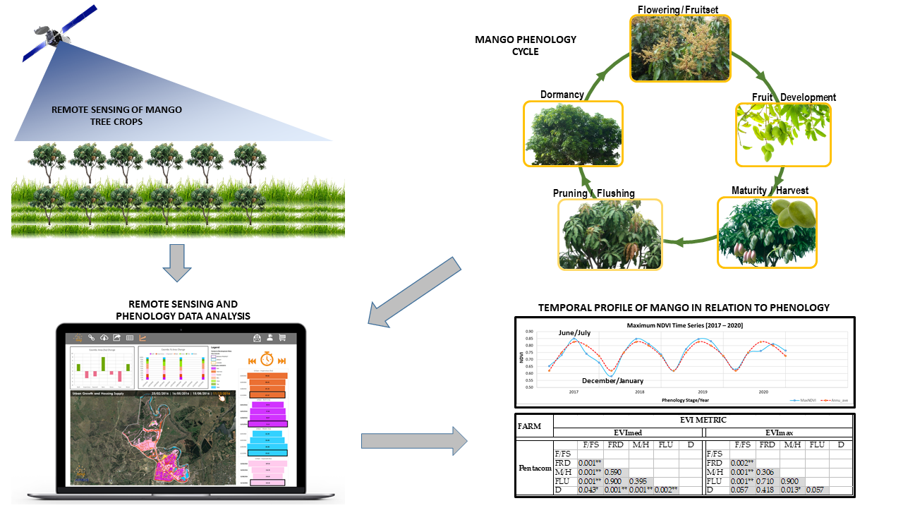
1. Introduction
2. Materials and Methods
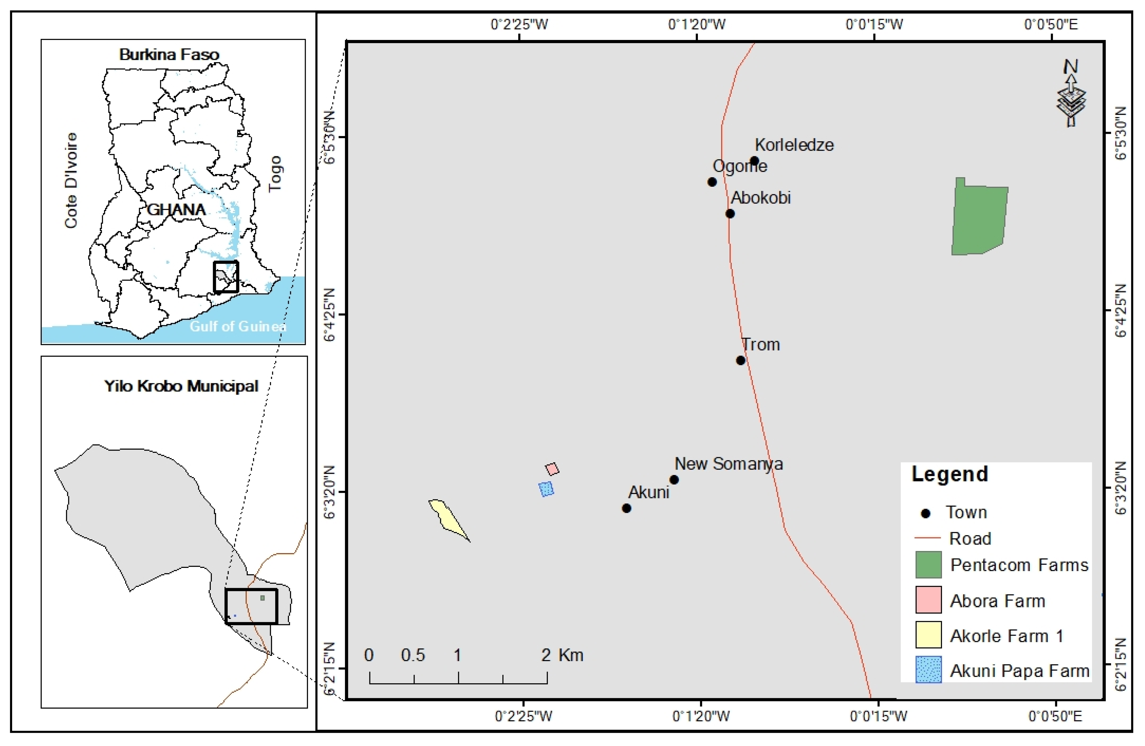
2.1. Study Area
2.2. Data Acquisition and Processing
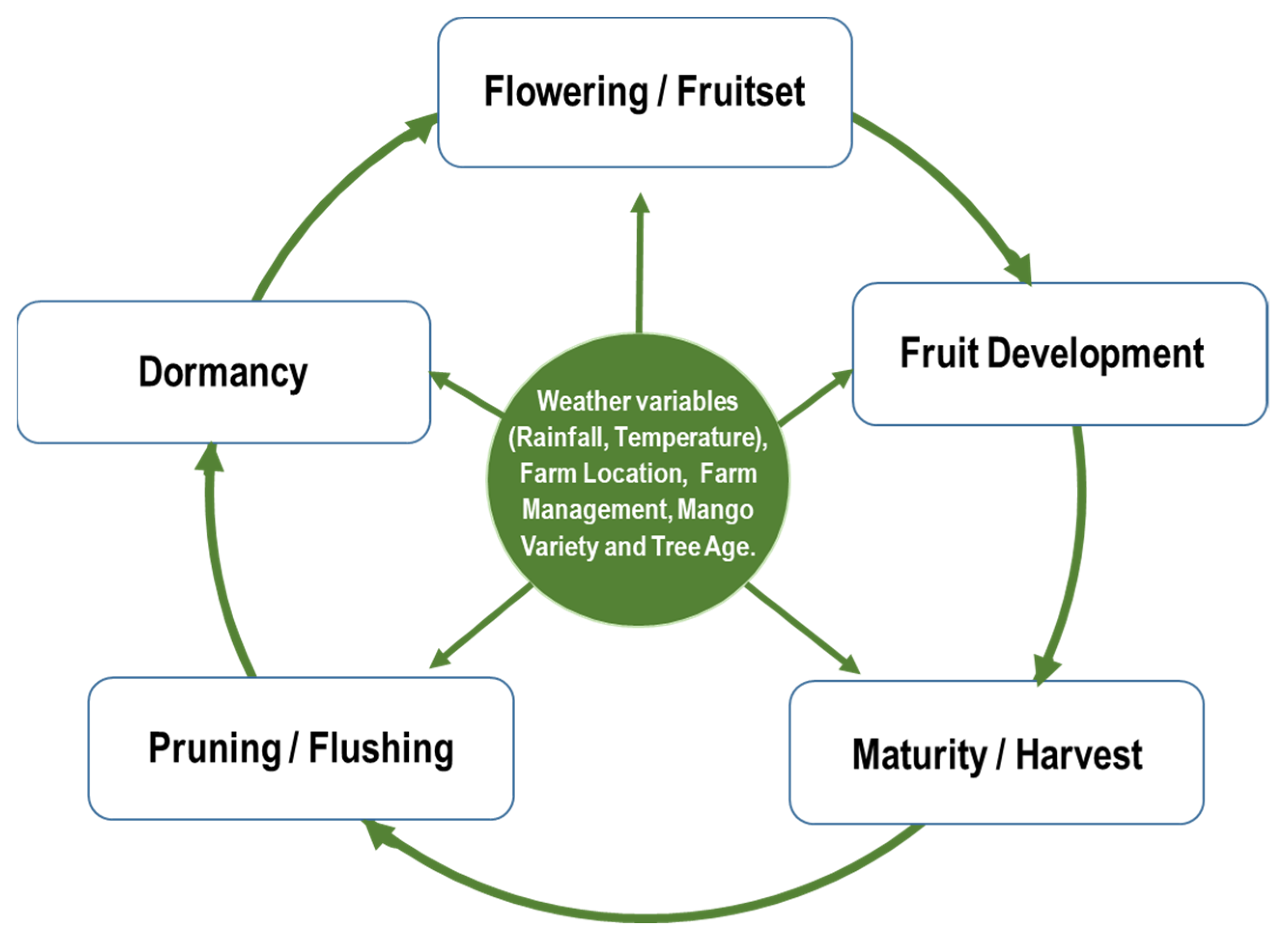
2.2.1. Mango Phenology Data
2.2.2. Extraction of Remote Sensing Data and Derivation of Vegetation Indices
2.3. Data Analysis
3. Results
3.1. Temporal Profiles of Remote Sensing Data at Key Phenological Stages
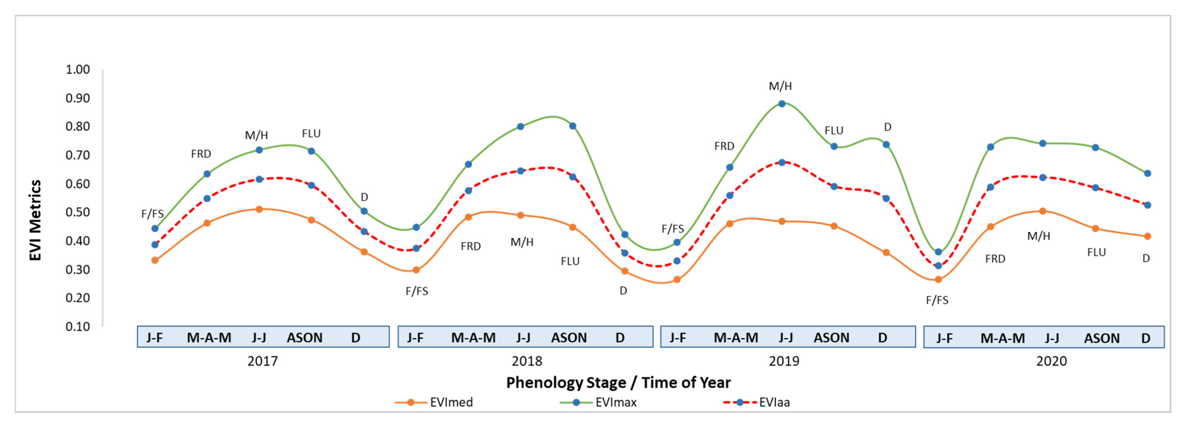
3.1.1. Pentacom Farm
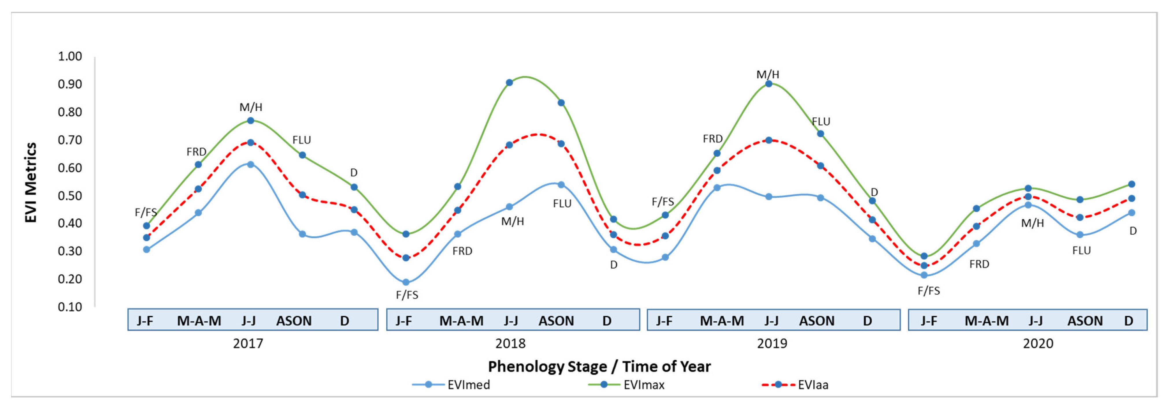
3.1.2. Abora Farm
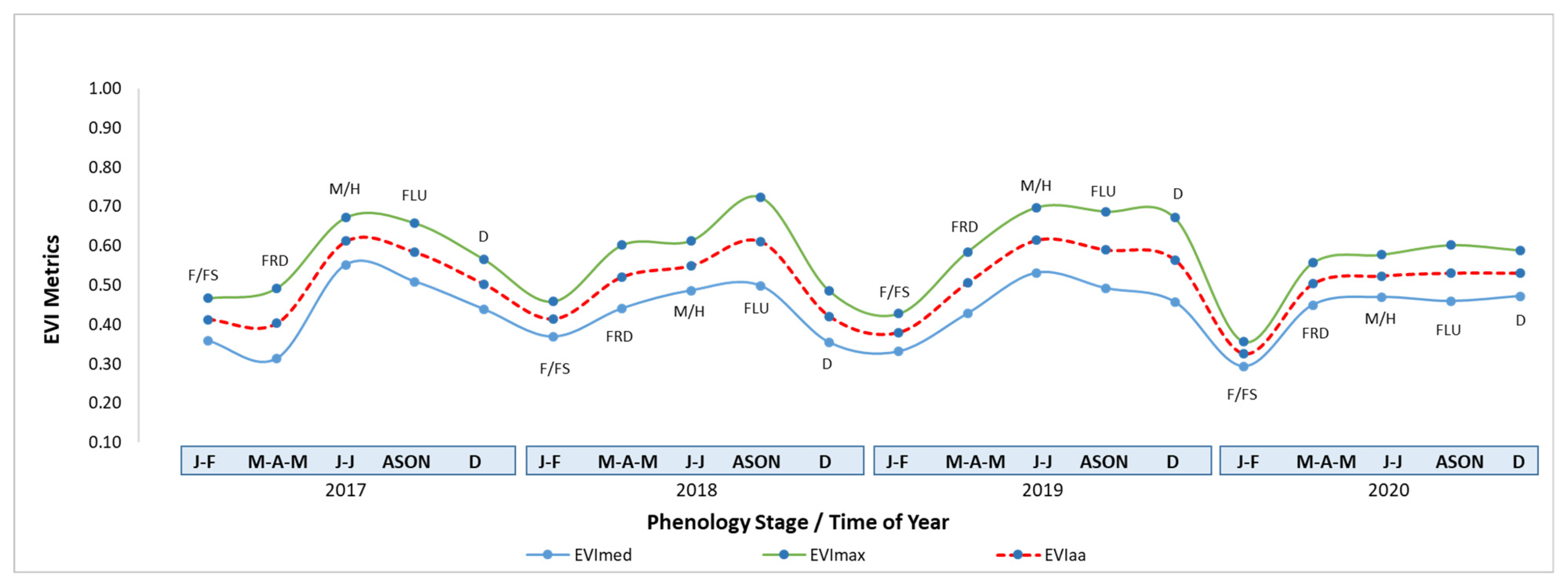
3.1.3. Akuni Papa Farm
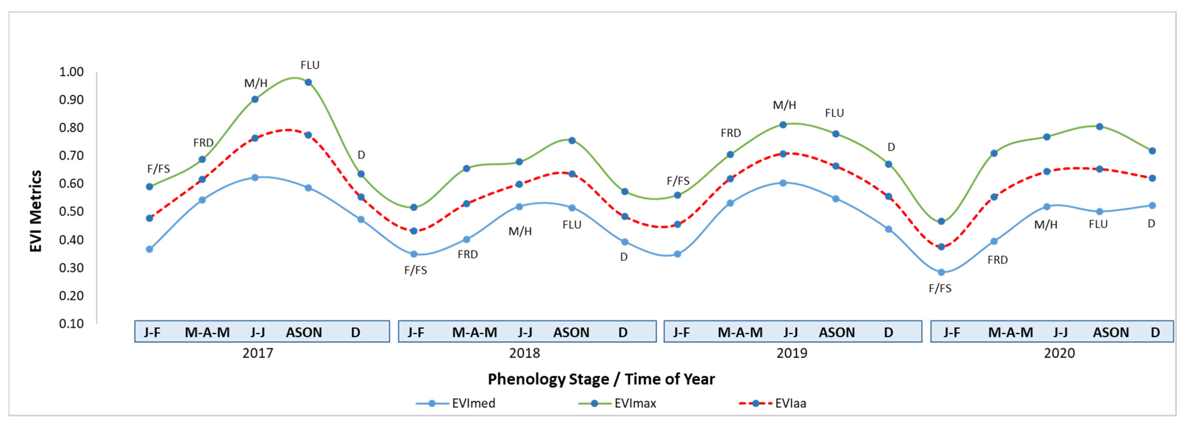
3.1.4. Akorle Farm 1
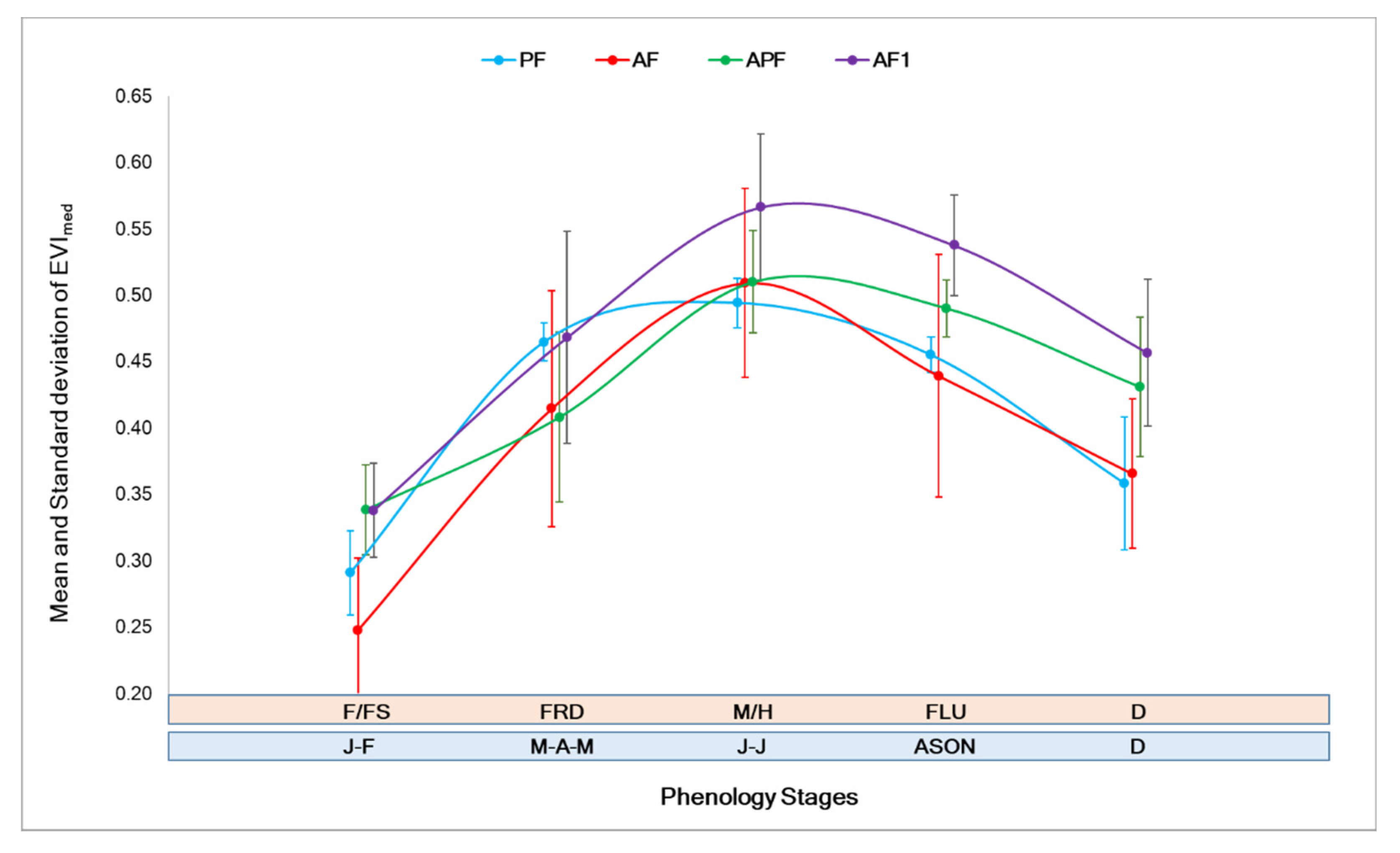
3.2. Temporal Variability of Mango Phenology within Farms
3.3. Temporal Variability of Mango Phenology between Farms
4. Discussion
5. Conclusions
Supplementary Materials
Author Contributions
Funding
Institutional Review Board Statement
Informed Consent Statement
Data Availability Statement
Acknowledgments
Conflicts of Interest
References
- Mahajan, G.R.; Das, B.; Murgaokar, D.; Herrmann, I.; Berger, K.; Sahoo, R.; Patel, K.; Desai, A.; Morajkar, S.; Kulkarni, R.M. Monitoring the Foliar Nutrients Status of Mango Using Spectroscopy-Based Spectral Indices and PLSR-Combined Machine Learning Models. Remote Sens. 2021, 13, 641. [Google Scholar] [CrossRef]
- FAOSTAT. Food and Agriculture Organization of the United Nations (FAO), FAO Statistic Database; FAOSTAT: Rome, Italy, 2021. [Google Scholar]
- Okorley, E.L.; Acheampong, L.; Abenor, M.T. The current status of mango farming business in Ghana: A case study of mango farming in the Dangme West District. Ghana J. Agric. Sci. 2014, 47, 73–80. [Google Scholar]
- Altendorf, S. Major Tropical Fruits Market Review 2017; FAO: Rome, Italy, 2019; p. 10. [Google Scholar]
- Evans, E.A.; Ballen, F.H.; Siddiq, M. Mango production, global trade, consumption trends, and postharvest processing and nutrition. In Handbook of Mango Fruit; John Wiley & Sons: Chichester, UK, 2017; pp. 1–16. [Google Scholar]
- Litz, R.E. The Mango: Botany, Production and Uses; Cabi: Wallingford, UK, 2009. [Google Scholar]
- Akotsen-Mensah, C.; Ativor, I.N.; Anderson, R.S.; Afreh-Nuamah, K.; Brentu, C.F.; Osei-Safo, D.; Boakye, A.A.; Avah, V. Pest Management Knowledge and Practices of Mango Farmers in Southeastern Ghana. J. Integr. Pest Manag. 2017, 8, 1–7. [Google Scholar] [CrossRef]
- Zakari, A. National Mango Study; International Trade Center: Geneva, Switzerland, 2012. [Google Scholar]
- Abu, M.; Olympio, N.; Darko, J.; Adu-Amankwa, P.; Dadzie, B. The mango industry in Ghana. Ghana J. Hortic. 2011, 9, 135–147. [Google Scholar]
- van Melle, C.; Buschmann, S. Comparative analysis of mango value chain models in Benin, Burkina Faso and Ghana. In Rebuilding West Africa’s Food Potential; FAO/IFAD: Rome, Italy, 2013. [Google Scholar]
- Inkoom, E.W.; Micah, J.A. Estimating Economic Efficiency of Mango Production in Ghana. ADRRI J. Agric. Food Sci. 2017, 3, 29–46. Available online: http://www.journals.adrri.org/ (accessed on 2 December 2021).
- Boakye-Yiadom, K.A.; Duca, D.; Pedretti, E.F.; Ilari, A. Environmental Performance of Chocolate Produced in Ghana Using Life Cycle Assessment. Sustainability 2021, 13, 6155. [Google Scholar] [CrossRef]
- Yidu, P.K.D.; Dzorgbo, D. The State and Mango Export Crop Production in Ghana. Ghana Soc. Sci. J. 2016, 13, 185–208. [Google Scholar]
- Ramirez, F.; Davenport, T.L.; Fischer, G.; Pinzón, J.C.A.; Ulrichs, C. Mango trees have no distinct phenology: The case of mangoes in the tropics. Sci. Hortic. 2014, 168, 258–266. [Google Scholar] [CrossRef]
- Zhao, G.; Gao, Y.; Gao, S.; Xu, Y.; Liu, J.; Sun, C.; Liu, S.; Chen, Z.; Jia, L.; Gao, Y.; et al. The Phenological Growth Stages of Sapindus mukorossi According to BBCH Scale. Forests 2019, 10, 462. [Google Scholar] [CrossRef] [Green Version]
- Delgado, P.M.H.; Aranguren, M.; Reig, C.; Galván, D.F.; Mesejo, C.; Fuentes, A.M.; Saúco, V.G.; Agustí, M. Phenological growth stages of mango (Mangifera indica L.) according to the BBCH scale. Sci. Hortic. 2011, 130, 536–540. [Google Scholar] [CrossRef]
- Rajan, S.; Tiwari, D.; Singh, V.; Saxena, P.; Reddy, S.S.Y.; Upreti, K.; Burondkar, M.; Bhagwan, A.; Kennedy, R. Application of extended BBCH Scale for phenological studies in mango (Mangifera indica L.). J. Appl. Hortic. 2011, 13, 108–114. [Google Scholar] [CrossRef]
- Siddiq, M.; Brecht, J.K.; Sidhu, J.S. Handbook of Mango Fruit: Production, Postharvest Science, Processing Technology and Nutrition; John Wiley & Sons: Hoboken, NJ, USA, 2017. [Google Scholar]
- Whiley, A.W. Environmental Effects on Phenology and Physiology of Mango—A Review. Acta Hortic. 1993, 341, 168–176. [Google Scholar] [CrossRef]
- Brunsell, N.; Pontes, P.P.B.; Lamparelli, R.A.C. Remotely Sensed Phenology of Coffee and Its Relationship to Yield. GISci. Remote Sens. 2009, 46, 289–304. [Google Scholar] [CrossRef]
- Baloch, M.K.; Bibi, F. Effect of harvesting and storage conditions on the post harvest quality and shelf life of mango (Mangifera indica L.) fruit. S. Afr. J. Bot. 2012, 83, 109–116. [Google Scholar] [CrossRef] [Green Version]
- Sivakumar, D.; Jiang, Y.; Yahia, E.M. Maintaining mango (Mangifera indica L.) fruit quality during the export chain. Food Res. Int. 2011, 44, 1254–1263. [Google Scholar] [CrossRef]
- Gianguzzi, G.; Farina, V.; Inglese, P.; Rodrigo, M.G.L. Effect of Harvest Date on Mango (Mangifera indica L. Cultivar Osteen) Fruit’s Qualitative Development, Shelf Life and Consumer Acceptance. Agronomy 2021, 11, 811. [Google Scholar] [CrossRef]
- Jha, S.; Narsaiah, K.; Sharma, A.; Singh, M.; Bansal, S.; Kumar, R. Quality parameters of mango and potential of non-destructive techniques for their measurement—A review. J. Food Sci. Technol. 2010, 47, 1–14. [Google Scholar] [CrossRef] [Green Version]
- Jha, S.; Kingsly, A.; Chopra, S. Physical and mechanical properties of mango during growth and storage for determination of maturity. J. Food Eng. 2006, 72, 73–76. [Google Scholar] [CrossRef]
- Prasad, K.; Jacob, S.; Siddiqui, M.W. Fruit maturity, harvesting, and quality standards. In Preharvest Modulation of Postharvest Fruit and Vegetable Quality; Academic Press: Cambridge, MA, USA, 2018; pp. 41–69. [Google Scholar]
- Ceglar, A.; van der Wijngaart, R.; de Wit, A.; Lecerf, R.; Boogaard, H.; Seguini, L.; Berg, M.V.D.; Toreti, A.; Zampieri, M.; Fumagalli, D.; et al. Improving WOFOST model to simulate winter wheat phenology in Europe: Evaluation and effects on yield. Agric. Syst. 2018, 168, 168–180. [Google Scholar] [CrossRef]
- Mouazen, A.M.; Kuang, B.; De Baerdemaeker, J.; Ramon, H. Comparison among principal component, partial least squares and back propagation neural network analyses for accuracy of measurement of selected soil properties with visible and near infrared spectroscopy. Geoderma 2010, 158, 23–31. [Google Scholar] [CrossRef]
- Krishna, G.; Sahoo, R.N.; Singh, P.; Bajpai, V.; Patra, H.; Kumar, S.; Dandapani, R.; Gupta, V.K.; Viswanathan, C.; Ahmad, T.; et al. Comparison of various modelling approaches for water deficit stress monitoring in rice crop through hyperspectral remote sensing. Agric. Water Manag. 2018, 213, 231–244. [Google Scholar] [CrossRef]
- Chemura, A.; Mutanga, O.; Odindi, J. Empirical modeling of leaf chlorophyll content in coffee (coffea arabica) plantations with sentinel-2 msi data: Effects of spectral settings, spatial resolution, and crop canopy cover. IEEE J. Sel. Top. Appl. Earth Obs. Remote Sens. 2017, 10, 5541–5550. [Google Scholar] [CrossRef]
- Wang, H.; Magagi, R.; Goïta, K.; Trudel, M.; McNairn, H.; Powers, J. Crop phenology retrieval via polarimetric SAR decomposition and Random Forest algorithm. Remote Sens. Environ. 2019, 231, 111234. [Google Scholar] [CrossRef]
- Zhang, H.; Kang, J.; Xu, X.; Zhang, L. Accessing the temporal and spectral features in crop type mapping using multi-temporal Sentinel-2 imagery: A case study of Yi’an County, Heilongjiang province, China. Comput. Electron. Agric. 2020, 176, 105618. [Google Scholar] [CrossRef]
- Küçük, Ç.; Taşkın, G.; Erten, E. Paddy-rice phenology classification based on machine-learning methods using multitemporal co-polar X-band SAR images. IEEE J. Sel. Top. Appl. Earth Obs. Remote Sens. 2016, 9, 2509–2519. [Google Scholar] [CrossRef]
- Ye, X.; Sakai, K.; Garciano, L.O.; Asada, S.-I.; Sasao, A. Estimation of citrus yield from airborne hyperspectral images using a neural network model. Ecol. Model. 2006, 198, 426–432. [Google Scholar] [CrossRef]
- Baret, F.; Weiss, M.; Troufleau, D.; Prevot, L.; Combal, B. Maximum information exploitation for canopy characterization by remote sensing. Asp. Appl. Biol. 2000, 60, 71–82. [Google Scholar]
- Koetz, B.; Baret, F.; Poilvé, H.; Hill, J. Use of coupled canopy structure dynamic and radiative transfer models to estimate biophysical canopy characteristics. Remote Sens. Environ. 2005, 95, 115–124. [Google Scholar] [CrossRef]
- Tedesco, D.; de Oliveira, M.F.; dos Santos, A.F.; Costa Silva, E.H.; de Souza Rolim, G.; da Silva, R.P. Use of remote sensing to characterize the phenological development and to predict sweet potato yield in two growing seasons. Eur. J. Agron. 2021, 129, 126337. [Google Scholar] [CrossRef]
- Kawamura, K.; Mackay, A.; Tuohy, M.P.; Betteridge, K.; Sanches, I.; Inoue, Y. Potential for spectral indices to remotely sense phosphorus and potassium content of legume-based pasture as a means of assessing soil phosphorus and potassium fertility status. Int. J. Remote Sens. 2011, 32, 103–124. [Google Scholar] [CrossRef]
- Darvishzadeh, R.; Skidmore, A.; Schlerf, M.; Atzberger, C.; Corsi, F.; Cho, M. LAI and chlorophyll estimation for a heterogeneous grassland using hyperspectral measurements. ISPRS J. Photogramm. Remote Sens. 2008, 63, 409–426. [Google Scholar] [CrossRef]
- Huete, A.; Didan, K.; van Leeuwen, W.; Miura, T.; Glenn, E. MODIS vegetation indices. In Land Remote Sensing and Global Environmental Change; Springer: Berlin/Heidelberg, Germany, 2010; pp. 579–602. [Google Scholar]
- Berger, K.; Verrelst, J.; Féret, J.-B.; Wang, Z.; Wocher, M.; Strathmann, M.; Danner, M.; Mauser, W.; Hank, T. Crop nitrogen monitoring: Recent progress and principal developments in the context of imaging spectroscopy missions. Remote Sens. Environ. 2020, 242, 111758. [Google Scholar] [CrossRef]
- Ferwerda, J.G.; Skidmore, A.K.; Mutanga, O. Nitrogen detection with hyperspectral normalized ratio indices across multiple plant species. Int. J. Remote Sens. 2005, 26, 4083–4095. [Google Scholar] [CrossRef]
- Lillesand, T.; Kiefer, R.W.; Chipman, J. Remote Sensing and Image Interpretation; John Wiley and Sons: Hoboken, NJ, USA, 2015. [Google Scholar]
- Blackburn, G.A. Hyperspectral remote sensing of plant pigments. J. Exp. Bot. 2006, 58, 855–867. [Google Scholar] [CrossRef] [Green Version]
- Nagaraja, A.; Sahoo, R.N.; Usha, K.; Singh, S.K.; Sivaramanae, N.; Gupta, V.K. Spectral discrimination of healthy and malformed mango panicles using spectrodariometer. Indian J. Hortic. 2014, 71, 40–44. [Google Scholar]
- Xue, J.; Su, B. Significant Remote Sensing Vegetation Indices: A Review of Developments and Applications. J. Sens. 2017, 2017, 1353691. [Google Scholar] [CrossRef] [Green Version]
- Avtar, R.; Yunus, A.P.; Saito, O.; Kharrazi, A.; Kumar, P.; Takeuchi, K. Multi-temporal remote sensing data to monitor terrestrial ecosystem responses to climate variations in Ghana. Geocarto Int. 2020, 1–17. [Google Scholar] [CrossRef]
- Wang, J.; Ding, J.; Yu, D.; Teng, D.; He, B.; Chen, X.; Ge, X.; Zhang, Z.; Wang, Y.; Yang, X.; et al. Machine learning-based detection of soil salinity in an arid desert region, Northwest China: A comparison between Landsat-8 OLI and Sentinel-2 MSI. Sci. Total Environ. 2020, 707, 136092. [Google Scholar] [CrossRef] [PubMed]
- Zeng, L.; Wardlow, B.D.; Wang, R.; Shan, J.; Tadesse, T.; Hayes, M.J.; Li, D. A hybrid approach for detecting corn and soybean phenology with time-series MODIS data. Remote Sens. Environ. 2016, 181, 237–250. [Google Scholar] [CrossRef]
- Hatfield, J.L.; Prueger, J.H. Value of Using Different Vegetative Indices to Quantify Agricultural Crop Characteristics at Different Growth Stages under Varying Management Practices. Remote Sens. 2010, 2, 562–578. [Google Scholar] [CrossRef] [Green Version]
- Suresh, K.; Behera, S.K.; Manorama, K.; Mathur, R.K. Phenological stages and degree days of oil palm crosses grown under irrigation in tropical conditions. Ann. Appl. Biol. 2020, 178, 121–128. [Google Scholar] [CrossRef]
- Sawant, S.A.; Chakraborty, M.; Suradhaniwar, S.; Adinarayana, J.; Durbha, S.S. Time Series Analysis of Remote Sensing Observations for Citrus Crop Growth Stage and Evapotranspiration Estimation. ISPRS—Int. Arch. Photogramm. Remote Sens. Spat. Inf. Sci. 2016, 41, 1037–1042. [Google Scholar] [CrossRef] [Green Version]
- Brinkhoff, J.; Vardanega, J.; Robson, A.J. Land Cover Classification of Nine Perennial Crops Using Sentinel-1 and -2 Data. Remote Sens. 2019, 12, 96. [Google Scholar] [CrossRef] [Green Version]
- Brinkhoff, J.; Robson, A.J. Block-level macadamia yield forecasting using spatio-temporal datasets. Agric. For. Meteorol. 2021, 303, 108369. [Google Scholar] [CrossRef]
- Vayssières, J.F.; Sinzogan, A.; Adandonon, A.; Rey, J.Y.; Dieng, E.O.; Camara, K.; Sangaré, M.; Ouedraogo, S.; Sidibé, A.; Keita, Y.; et al. Annual population dynamics of mango fruit flies (Diptera: Tephritidae) in West Africa: Socio-economic aspects, host phenology and implications for management. Fruits 2014, 69, 207–222. [Google Scholar] [CrossRef]
- Vannière, H.; Rey, J.-Y.; Vayssières, J.-F.; Maraite, H. Crop Production Protocol—Mango (Mangifera indica); PIP: Maastricht, The Netherlands, 2013. [Google Scholar]
- DEA. Digital Earth Africa User Guide. Available online: https://docs.digitalearthafrica.org/en/latest/data_specs/Sentinel-2_Level-2A_specs.html (accessed on 2 August 2021).
- Main-Knorn, M.; Pflug, B.; Louis, J.; Debaecker, V.; Müller-Wilm, U.; Gascon, F. Sen2Cor for sentinel-2. In Image and Signal Processing for Remote Sensing XXIII; International Society for Optics and Photonics: Bellingham, WA, USA, 2017; p. 1042704. [Google Scholar]
- Obregón, M.Á.; Rodrigues, G.; Costa, M.J.; Potes, M.; Silva, A.M. Validation of ESA Sentinel-2 L2A Aerosol Optical Thickness and Columnar Water Vapour during 2017–2018. Remote Sens. 2019, 11, 1649. [Google Scholar] [CrossRef] [Green Version]
- Gascon, F.; Bouzinac, C.; Thépaut, O.; Jung, M.; Francesconi, B.; Louis, J.; Lonjou, V.; Lafrance, B.; Massera, S.; Gaudel-Vacaresse, A.; et al. Copernicus Sentinel-2A Calibration and Products Validation Status. Remote Sens. 2017, 9, 584. [Google Scholar] [CrossRef] [Green Version]
- Richter, R.; Louis, J.; Müller-Wilm, U. Sentinel-2 MSI—Level 2A Products Algorithm Theoretical Basis Document; European Space Agency: Paris, France, 2012; Volume 49, pp. 1–72. [Google Scholar]
- Braaten, J.D.; Cohen, W.B.; Yang, Z. Automated cloud and cloud shadow identification in Landsat MSS imagery for temperate ecosystems. Remote Sens. Environ. 2015, 169, 128–138. [Google Scholar] [CrossRef] [Green Version]
- Zekoll, V.; Main-Knorn, M.; Alonso, K.; Louis, J.; Frantz, D.; Richter, R.; Pflug, B. Comparison of Masking Algorithms for Sentinel-2 Imagery. Remote Sens. 2021, 13, 137. [Google Scholar] [CrossRef]
- Zhu, Z.; Wang, S.; Woodcock, C.E. Improvement and expansion of the Fmask algorithm: Cloud, cloud shadow, and snow detection for Landsats 4–7, 8, and Sentinel 2 images. Remote Sens. Environ. 2015, 159, 269–277. [Google Scholar] [CrossRef]
- Rouse, J., Jr.; Haas, R.; Schell, J.; Deering, D. Monitoring Vegetation Systems in the Great Plains with Erts; NASA Special Publication: Washington, DC, USA, 1974; Volume 351, p. 309. [Google Scholar]
- Gitelson, A.A.; Gritz, Y.; Merzlyak, M.N. Relationships between leaf chlorophyll content and spectral reflectance and algorithms for non-destructive chlorophyll assessment in higher plant leaves. J. Plant Physiol. 2003, 160, 271–282. [Google Scholar] [CrossRef] [PubMed]
- Huete, A.; Didan, K.; Miura, T.; Rodriguez, E.P.; Gao, X.; Ferreira, L.G. Overview of the radiometric and biophysical performance of the MODIS vegetation indices. Remote Sens. Environ. 2002, 83, 195–213. [Google Scholar] [CrossRef]
- Kaufman, Y.J.; Justice, C.O.; Flynn, L.P.; Kendall, J.D.; Prins, E.M.; Giglio, L.; Ward, D.E.; Menzel, W.P.; Setzer, A.W. Potential global fire monitoring from EOS-MODIS. J. Geophys. Res. 1998, 103, 32215–32238. [Google Scholar] [CrossRef]
- Huete, A.R. A soil-adjusted vegetation index (SAVI). Remote Sens. Environ. 1988, 25, 295–309. [Google Scholar] [CrossRef]
- Rahman, M.M.; Robson, A.J. A Novel Approach for Sugarcane Yield Prediction Using Landsat Time Series Imagery: A Case Study on Bundaberg Region. Adv. Remote Sens. 2016, 5, 93–102. [Google Scholar] [CrossRef] [Green Version]
- Vani, V.; Mandla, V.R. Comparative Study of NDVI and SAVI vegetation Indices in Anantapur district semi-arid areas. Int. J. Civ. Eng. Technol. 2017, 8, 559–566. [Google Scholar]
- Wiegand, C.; Gerbermann, A.; Gallo, K.; Blad, B.; Dusek, D. Multisite analyses of spectral-biophysical data for corn. Remote Sens. Environ. 1990, 33, 1–16. [Google Scholar] [CrossRef]
- Wiegand, C.L.; Maas, S.J.; Aase, J.K.; Hatfield, J.L.; Pinter, P.J.; Jackson, R.D.; Kanemasu, E.T.; Lapitan, R.L. Multisite analyses of spectral-biophysical data for wheat. Remote Sens. Environ. 1992, 42, 1–21. [Google Scholar] [CrossRef]
- Yoav, B.; Braun, H.; John, W. Tukey’s Contributions to Multiple Comparisons. Ann. Stat. 2002, 30, 1576–1594. Available online: https://www.jstor.org/stable/1558730 (accessed on 9 November 2021).
- Vasavada, N. One-Way ANOVA with Post-Hoc Tukey HSD Test Calculator. Available online: https://astatsa.com/OneWay_Anova_with_TukeyHSD/_get_data/ (accessed on 1 July 2021).
- Jannoyer, M.; Lauri, P.-E. Young Flush Thinning in Mango (cv. Cogshall) Controls Canopy Density and Production. Acta Hortic. 2009, 820, 395–402. [Google Scholar] [CrossRef]
- Solanki, P.; Shah, N.; Sonavane, S.; Prajapati, D. Impact of different pruning time and intensity on vegetative parameters of mango cv. Kesar under high density plantation. Ecol. Environ. Conserv. 2014, 20, S411–S414. [Google Scholar]
- Kouadio, L.; Newlands, N.K.; Davidson, A.; Zhang, Y.; Chipanshi, A. Assessing the Performance of MODIS NDVI and EVI for Seasonal Crop Yield Forecasting at the Ecodistrict Scale. Remote Sens. 2014, 6, 10193–10214. [Google Scholar] [CrossRef] [Green Version]
- Anderson, L.O.; Aragão, L.E.O.C.; Shimabukuro, Y.E.; Almeida, S.; Huete, A. Fraction images for monitoring intra-annual phenology of different vegetation physiognomies in Amazonia. Int. J. Remote Sens. 2011, 32, 387–408. [Google Scholar] [CrossRef]
- Ovakoglou, G.; Alexandridis, T.K.; Clevers, J.G.P.W.; Gitas, I.Z. Downscaling of MODIS leaf area index using landsat vegetation index. Geocarto Int. 2020, 1–24. [Google Scholar] [CrossRef]
- Yebra, M.; Van Dijk, A.; Leuning, R.; Huete, A.; Guerschman, J.P. Evaluation of optical remote sensing to estimate actual evapotranspiration and canopy conductance. Remote Sens. Environ. 2013, 129, 250–261. [Google Scholar] [CrossRef]
- Basso, B.; Cammarano, D.; Carfagna, E. Review of Crop Yield Forecasting Methods and Early Warning Systems. In Proceedings of the First Meeting of the Scientific Advisory Committee of the Global Strategy to Improve Agricultural and Rural Statistics, Rome, Italy, 18 July 2013. [Google Scholar]
- Sadeh, Y.; Zhu, X.; Dunkerley, D.; Walker, J.P.; Zhang, Y.; Rozenstein, O.; Manivasagam, V.; Chenu, K. Fusion of Sentinel-2 and PlanetScope time-series data into daily 3 m surface reflectance and wheat LAI monitoring. Int. J. Appl. Earth Obs. Geoinf. 2020, 96, 102260. [Google Scholar] [CrossRef]


| Name of Farm | Location | Ownership/Management | Coordinate of Centroid | Tree Age (yr) | Size (ha) | Spacing (m) | Variety (%) |
|---|---|---|---|---|---|---|---|
| Pentacom Farms | Somanya | Corporate | 0°0′22.045″ E 6°4′59.591″ N | 18 | 45.0 | 10 × 8 | Keitt (85), Kent and Others (15) |
| Abora Farm | Somanya | Small grower | 0°2′14.438″ W 6°3′28.195″ N | 18 | 1.3 | 10 × 10 | Keitt (95), Kent (5) |
| Akuni Papa Farm | Somanya | Small grower | 0°2′16.705″ W 6°3′20.774″ N | 18 | 1.9 | 9 × 9 | Keitt (95), Kent (5) |
| Akorle Farm 1 | Somanya | Small grower | 0°2′53.204″ W 6°3′10.632″ N | 18 | 6.0 | 10 × 10 | Keitt (95), Kent (5) |
| NDVI Metrics | GNDVI Metrics | EVI Metrics | SAVI Metrics | ||||||
|---|---|---|---|---|---|---|---|---|---|
| FARM | Significance Test | Median | Maximum | Median | Maximum | Median | Maximum | Median | Maximum |
| PF | p-value | 0.0004 | 4.2 × 10⁻⁶ | 0.0376 | 0.0013 | 2.3 × 10⁻⁷ | 3.9 × 10⁻⁵ | 5.3 × 10⁻⁵ | 4.8 × 10⁻⁶ |
| AF | p-value | 0.2752 | 2.2 × 10⁻¹ | 0.3068 | 0.1610 | 2.3 × 10⁻³ | 1.8 × 10⁻³ | 5.9 × 10⁻² | 3.5 × 10⁻² |
| AF1 | p-value | 0.0017 | 4.7 × 10⁻⁷ | 0.0040 | 0.0008 | 3.2 × 10⁻⁴ | 2.3 × 10⁻⁴ | 1.2 × 10⁻³ | 1.6 × 10⁻⁴ |
| APF | p-value | 0.2730 | 2.7 × 10⁻¹ | 0.3426 | 0.3480 | 5.1 × 10⁻⁴ | 2.6 × 10⁻⁴ | 2.1 × 10⁻² | 1.8 × 10⁻² |
| FARM | EVI METRIC | |||||||||||
|---|---|---|---|---|---|---|---|---|---|---|---|---|
| EVImed | EVImax | |||||||||||
| Pentacom | F/FS | FRD | M/H | FLU | D | F/FS | FRD | M/H | FLU | D | ||
| F/FS | ||||||||||||
| FRD | 0.001 ** | 0.002 ** | ||||||||||
| M/H | 0.001 ** | 0.590 | 0.001 ** | 0.306 | ||||||||
| FLU | 0.001 ** | 0.900 | 0.395 | 0.001 ** | 0.710 | 0.900 | ||||||
| D | 0.043 * | 0.001 ** | 0.001 ** | 0.002 ** | 0.057 | 0.418 | 0.013 * | 0.057 | ||||
| Abora | F/FS | |||||||||||
| FRD | 0.041 * | 0.177 | ||||||||||
| M/H | 0.001 ** | 0.402 | 0.001 ** | 0.544 | ||||||||
| FLU | 0.018 * | 0.900 | 0.631 | 0.014 * | 0.111 | 0.900 | ||||||
| D | 0.201 | 0.885 | 0.097 | 0.657 | 0.024 * | 0.624 | 0.705 | 0.225 | ||||
| Akuni Papa | F/FS | |||||||||||
| FRD | 0.242 | 0.037 * | ||||||||||
| M/H | 0.001 ** | 0.042 * | 0.001 ** | 0.313 | ||||||||
| FLU | 0.002 ** | 0.129 | 0.900 | 0.001 ** | 0.104 | 0.900 | ||||||
| D | 0.075 | 0.900 | 0.147 | 0.378 | 0.014 * | 0.900 | 0.571 | 0.237 | ||||
| Akorle Farm 1 | F/FS | |||||||||||
| FRD | 0.031 * | 0.051 | ||||||||||
| M/H | 0.001 ** | 0.130 | 0.001 ** | 0.282 | ||||||||
| FLU | 0.001 ** | 0.359 | 0.900 | 0.001 ** | 0.096 | 0.900 | ||||||
| D | 0.057 | 0.900 | 0.073 | 0.222 | 0.191 | 0.900 | 0.081 | 0.0235 * | ||||
| NDVI | GNDVI | EVI | SAVI | |||||
|---|---|---|---|---|---|---|---|---|
| Median | Maximum | Median | Maximum | Median | Maximum | Median | Maximum | |
| Phenology Stage | 3.1 × 10⁻⁶ | 6.4 × 10⁻⁷ | 3.2 × 10⁻⁶ | 5.1 × 10⁻⁶ | 4.4 × 10⁻⁷ | 1.3 × 10⁻⁶ | 2.4 × 10⁻⁷ | 2.2 × 10⁻⁶ |
| Mango Farm | 2.3 × 10⁻⁶ | 9.8 × 10⁻⁷ | 3.6 × 10⁻⁵ | 9.5 × 10⁻⁵ | 2.0 × 10⁻³ | 1.5 × 10⁻³ | 3.3 × 10⁻⁴ | 5.1 × 10⁻⁴ |
Publisher’s Note: MDPI stays neutral with regard to jurisdictional claims in published maps and institutional affiliations. |
© 2021 by the authors. Licensee MDPI, Basel, Switzerland. This article is an open access article distributed under the terms and conditions of the Creative Commons Attribution (CC BY) license (https://creativecommons.org/licenses/by/4.0/).
Share and Cite
Torgbor, B.A.; Rahman, M.M.; Robson, A.; Brinkhoff, J.; Khan, A. Assessing the Potential of Sentinel-2 Derived Vegetation Indices to Retrieve Phenological Stages of Mango in Ghana. Horticulturae 2022, 8, 11. https://doi.org/10.3390/horticulturae8010011
Torgbor BA, Rahman MM, Robson A, Brinkhoff J, Khan A. Assessing the Potential of Sentinel-2 Derived Vegetation Indices to Retrieve Phenological Stages of Mango in Ghana. Horticulturae. 2022; 8(1):11. https://doi.org/10.3390/horticulturae8010011
Chicago/Turabian StyleTorgbor, Benjamin Adjah, Muhammad Moshiur Rahman, Andrew Robson, James Brinkhoff, and Azeem Khan. 2022. "Assessing the Potential of Sentinel-2 Derived Vegetation Indices to Retrieve Phenological Stages of Mango in Ghana" Horticulturae 8, no. 1: 11. https://doi.org/10.3390/horticulturae8010011