The Journal of Science Extension Research – Vol. 3, 2024

Image credits

Cover : Jayden Sandison, Illawarra Sports High School

A homemade wind tunnel setup used to accurately measure the lifting force on wings of different shapes and to study how air flows over them at different angles .

Inside cover : Munjir Anoar, Girraween High School

This graph shows how the amount of light received by a planet (insolation flux) changes with the proportion of heavy elements (stellar metallicity) within the star it orbits

FOREWORD

I am honoured to write the foreword to this volume of the Journal of Science Extension Research. Science Extension is a truly innovative Stage 6 science course that pushes the boundaries of science education in schools. The course is designed to enable its students to experience authentic science and the captivation of engaging in scientificinquiryof the natural world. For them, science is not limited to the content of textbooks or the walls of their classrooms.

Thegoal of equity in education meansensuring every student can access the resources, opportunities and support they need to achieve their full potential. As I read through the articles in this Journal, I was struck by the diversity of the schools and students represented and the acknowledgment of the support they have received from their teachers, peers, academic mentors, research scientists, and institutions. I am proud of their achievements and appreciate how public education has empowered them to excel.

The articles in this Journal highlight the excellence our students can attain. The range of topics the students investigated is impressive, spanning fieldssuch asbiomedical sciences,astronomy, mathematical modelling and computer simulations. What unitesthem all istheir focuson scientific inquiryand thepursuit of evidence-based answers toquestions.

The research outputs showcase the work of the brilliant young minds who have completed their Science Extension journeys. Those journeys were only possible through the efforts and expertise of their Science Extension teachers. These dedicated teachers guide their students to complete research projectsand producescientificreportsthat resemble authenticscientificjournal articles.Congratulations

Murat Dizdar PSM Secretary of the NSW Department of Education

The achievements of Science “ Extension teachers and students exemplifythevalues of public education asdescribed in the Plan for NSW Public Education.

“

Science Extension teachers for taking on the monumental task of teaching the course and inspiring the next generation of STEM professionals.

It is a pleasure to note the positive impact that the Journal is having on science education. The articles in theJournal not onlyshowcaseexcellencein studentled scientificresearch but areused asinstructional resources in science classrooms. Notably, the work of some Science Extension students has been featured in competitions such as the Young Scientist Awards and the International Science and Engineering Fair.

The achievements of Science Extension teachers and students exemplify the values of public education as described in the Plan for NSW Public Education. Passionate students, led by courageous teachers, probeand question phenomena todiscover scientific explanations of the Universe to which we belong. In doing so, these apprentice scientists are taking their first steps in addressing global issuesand constructing an optimistic future. They join the ranks of the many STEM professionals who ensure Australia is at the forefront of creating that future. I congratulate the Science Extension students whose work is contained in this volume of the Journal of Science Extension Research. I also wish the future cohorts of the Science Extension coursethebest in their scientificendeavours.

Tobie White

Armidale Secondary College

School has always aimed to prepare students for the real world, offering courses that develop the skills they may need to succeed in certain careers – hospitality, visual arts, sport science and so on. However, there had long been a gap in preparing studentsfor scientificresearch.Manystudents struggled in higher education because of this. For example,when I did first year statisticsat university, only 40% passed, partly due to poor preparation in high school. The Science Extension coursefillsthisneed.It uniquelyprepares students for a world of research, teaching them data collection and analysis, collaboration, critical and creative thinking, using various technologies and problem solving.

I have taught the course since its inception, helping a range of students achieve their academic goals. Some of our school’s highest results were achieved by students undertaking Science Extension, many of whom have gone on to study medicine and engineering at university. I have also had students who had otherwise struggled in science join the course because of their love of science and thirst for the skills and knowledge included in this course was so great that they could not be dissuaded. I am glad for this, with onesuch student being thefirst person in their family to complete the HSC. ‘Extension’ means different things to different people, for example, the level to which your science knowledge and skills can be extended may be different to mine. This course isn’t just for students who present as academically gifted or those who will achieve the highest results; it is for those with passion, those who seek answers, those who want to extend themselves. Keep this in mind when promoting the course each year.

“ make it interesting and make sure it isdoable

“My advice to those teaching the course; try to get out of theway.Onceyou light thefirein thebellies of your students and give them the basic knowledge and skillstoinvestigatetheir own question,let them go and do science. As a teacher, it can be hard not to manage every step along the way, but too much control subtracts more from the student’s learning experience than it adds. Guide them and teach them the skills they need (especially data analysis and interpretation), but ultimately let them take charge and do science.

My advice to students undertaking the course; make it interesting and make sure it is doable. Make it interesting to you, after all you are the one who will be doing the project. There will always be others whofind your topicinteresting,and theywill seek you out in time. Make sure you can actually do your project; doyou havethedata or equipment totest your variable? Start with an idea and figureout what is achievable by seeing what research is out there, what data theyhaveand what equipment you have. Your inquiryquestion will refineitself over thefirst few months as you do this–don’t be put off by this, it is normal. Remember, you can investigate your topic in more detail at university.

I would encourage everyone to really read through the wonderful research papers submitted here. They are the product of passion, and the culmination of many hours of hard work by dedicated students looking to extend themselves in some way.

ACKNOWLEDGEMENTS

This edition includes research reports from Science Extension students who completed the course in 2023. All reports are the work of students studying in NSW public schools. They have been supported by their teachers and schools, and in some cases, external mentors.

TheScience7-12 curriculum team acknowledgestheincredible efforts of Science Extension teachers in inspiring, guiding and mentoring their studentstocompletetheir scientificresearch projects. Despite the novelty and innovativeness of the syllabus, those teachers spared no effort to nurture their students’ scientificcuriosityand engagethem in conducting authentic scientificinquiry.As a result,their studentshaveexperienced newheightsof academicand scientificachievementsin their research journeys.

To all NSW Department of Education schools, we thank you for your sustained efforts in achieving excellence in scienceeducation.

ACKNOWLEDGEMENTS

We acknowledge the following teachers whose students’ reports appear in this publication:

• George An, Ryde Secondary College

• Ritu Bhamra, Normanhurst Boys High School

• Joshua Bowles, James Cook Boys Technology High School

• Sally Chahine, Sir Joseph Banks High School

• Deb Chaudhuri, Turramurra High School

• Carina Dennis, James Ruse Agricultural High School

• Sally Doig, Leeton High School

• Milena Driscoll, Barrenjoey High School

• Wade Fairclough, Cherrybrook Technology High School

• Angela Foy, Gosford High School

• Louis Green, Girraween High School

• Marina Gulline, Willoughby Girls High School

• Ann Hanna, Menai High School

• Vero Joseph, Crookwell High School

• Kurt Nicholson, Lambton High School

• Joelle Rodrigues, Blacktown Girls High School

• Dr Samantha Kneeshaw, Ulladulla High School

• Erika Savage, Peel High School

• Karin Schaffarczyk McHale, Northmead Creative and Performing Arts High School

• Kyle Strano, Grafton High School

• Andrew Tann, Inverell High School

• Margaret Thomas, Illawarra Sports High School

• Michelle Tory, Coffs Harbour Senior College

• Tobie White, Armidale Secondary College

• Leigh Wood, Wollumbin High School

Showcasing excellence in Science Extension

Showcasing excellence in Science Extension

Project overview

To support the Science Extension course, the Science7-12 curriculum teamhasinitiated a project to document students’, teachers’ and mentors’ experiencesengaging in theScientificResearch Project. To that end, the team has produced the following outputs:

• A series of videos featuring current and exScience Extension students, teachers and mentors. They show great ways to teach and learn, including inspirational messages from teachers and students.

• The Journal of Science Extension Research explores the different topics and types of investigations completed by students, celebrating their research achievements in the course.

In addition, Olivia Clarkson, under the supervision of Bonnie McBain and Liam Phelan at the University of Newcastle, analysed the value of the Science Extension course in promoting excellence in science education. Her research material included the video resources produced in this project. Their report is included as an invited paper in this volume of the Journal.

These resources enhance teachers’ pedagogical content knowledge of the subject, providing diverse examples of effective teaching and learning and recognising students’ achievements in NSW public schools.

Video resources

Stagesof the Scientific Research Project

The first sequenceof videos builds an understanding of thestagesin developing theScientificResearch Project.

• Getting started, conducting a lit review

• Collecting the processing data

• Writing a great report

Supporting progress

Teachers, students and mentors outline the challenges they experienced, and strategies for progressing their Scientific Research Project.

• Planning to achieve

• Building a science extension program

• The mentoring process

Student profiles

Past studentsreflect on their research experience in Science Extension.

• Student profile– Montana

• Student profile– Sarah

• Student profile–Vincent

IN THIS EDITION

28 – 38

Invited paper

Evaluating Science Extension: Perspectives from the literature, teachers, students and mentors

Olivia Clarkson, Third-year student, Bachelor of Science (Advanced), University of Newcastle Thisstudy evaluates thequality of education provided by theScience Extension course. The evaluation includes scientific literature, department documents and analysis of interviews with students, teachers, and mentors. The course meets its educational objectives, effectively facilitating learning in project-based learning, relevance, statistics, collaboration, and passion. Thissuggests that thecourse’s structure and focus on student-centred learning and practical skills are effective in enhancing science education in the HSC program.

39 –57

The truth of aspartame’s impact on body and health

Ariel Belic, Barrenjoey High School

The study aims to analyse existing research on aspartame’s effects on body weight and cancer risk. It was found that regular aspartame consumption does not contribute to adverse health effects, such as significant bodymass changes or an elevated cancer risk and may to assist in long-term weight management, albeit with a minimal impact. These findings suggest therelative safety of regular aspartame intake, highlighting its potential utility in dietary control. However, extensive, well-controlled future research, incorporating diverse human subjects isrequired to fully comprehend aspartame’s long-term health effects.

58 – 69

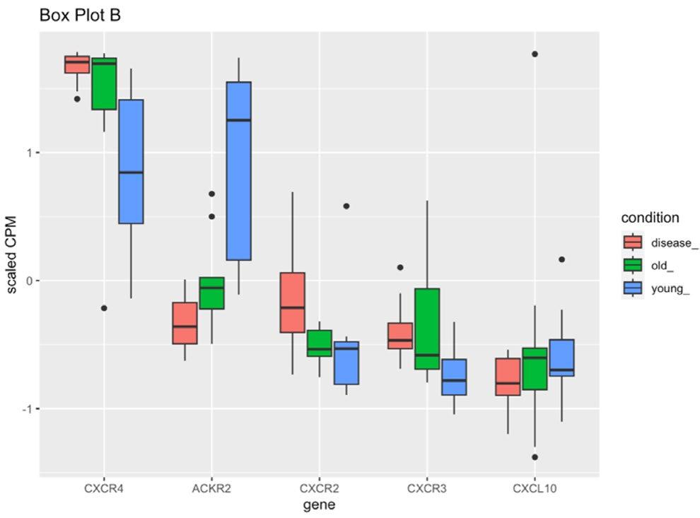
A differential expression analysisof chemokine receptor binding genes between RNA sequencing datasetsof Alzheimer and non-Alzheimer patients

Kenny Cao, Normanhurst Boys High School

The paper analysed differential gene expression related to chemokine receptor binding in Alzheimer’s patients versus non-affected individuals. Five genes, especially CXCL10 and CXCR3, showed significant differential expression, potentially serving as biomarkers or therapeutic targets. These findings pave theway for novel Alzheimer’s treatments and diagnostic strategies, demonstrating the role of specific genes in disease progression.

IN THIS EDITION

70 – 77

Contributors to success in volleyball matches: The effect of servereception on the outcome of a high school volleyball match

David Chang, Ryde Secondary College

Thestudy aimed to ascertain theimpact of serve-reception on theoutcomes of high school volleyball matches. Thestudy assessed how different types of passes influenced match outcomes by analysing videofootage of serve-receive actions across various high-level competitions. The analysis concluded that thequality of serve-receive directly influences points won or lost, thereby affecting theoverall match result. Emphasising serve-reception skills during training could significantly enhance a team’s success rate in volleyball matches.

78 – 87

The relationship between germline mutations and the incidence rate of pancreatic cancer

Bronte Elliott, Wollumbin High School

The research examines how certain germline mutation affect pancreatic cancer’s incidence and progression. Significant genetic differences were noted between groups, with 21.9% of PC subjects exhibiting selected germline mutations, com-pared to 2.6% of non-PC participants. These insights highlight the roll of heredity in pancreatic cancer, suggesting that early screening for these mutations could enhance diagnosis, improve prognosis and inform genetic counselling.

88 – 101

Raising the alarm bells on antimicrobial resistance

Holly Forbes, Ulladulla High School

Theresearch examines whether public awareness of Antimicrobial Resistance (AMR) influences themisuseof antibiotics and affects resistance trends. Awareness of AMR significantly correlates with reduced antibiotic misuse. However, awareness may not be the sole factor in resistance emergence, and Antimicrobial Stewardship (AMS) programs did not significantly affect antibiotic prescriptions. The study emphasises the importance of nationwide educational and AMS strategies across various health sectors to mitigate risks associated with AMR.

IN THIS EDITION

102 – 114

Factors that influence the risk of post-operativedelirium in general anesthesia patients

Rosalie Gibbs, Northmead Creative and Performing Arts High School

To identify and understand the factors that increase the likelihood of Postoperative Delirium (POD) following general anaesthesia. Age, sex, and pre-existing cognitive dysfunction significantly influence therisk of POD, with older age and male gender being particularly associated with increased risk.These insights are crucial for pre-operative assessments, allowing for personalised patient care strategies and improved post-operative outcomes through early diagnosis and treatment of POD.

115 – 122

Bichordal harmonic musical intervals and effects on overall satisfaction

Joshua Gibson, Ryde Secondary College

Thestudy aimed to determine if different bichordal harmonic intervals (BI’s) influence listener satisfaction levels. More consonant BI’s were found to besignificantly more satisfying than dissonant ones, with specific intervals identified as most and least satisfying. Understanding these preferences can guide music composition across genres and historical periods and inform sound design in public spaces to enhance well-being and productivity.

123 – 141

The effects of font and colour on text legibility

Ethan Ho, Ryde Secondary College

This study investigated how different fonts and colours affect the legibility of text. Sans serif fonts, specifically Arial, were found to bemore legible than serif fonts, with certain colour backgrounds enhancing legibility. However,not all colour pairings showed significant differences. Further research is needed to explore a broader range of colours and fonts, aiming for consistent data across the spectrum to enhance text legibility in various media.

IN THIS EDITION

142 – 161

Theeffect static and dynamic stretching haveon hamstring flexibility

Madeline Irvin, Leeton High School

This study aims to identify which form of stretching, static or dynamic, is more effective in enhancing hamstring flexibility, a key factor in athletic performance and injury prevention. The study found that dynamicstretching led to greater improvements in hamstring flexibility.However, external uncontrollable factors impacted the validity, and statistical analysis (ANOVA) showed no significant difference between thegroups. Thefindings suggest that while regular hamstring stretching is beneficial, further research is needed.

162 – 176

A comparative review of miR-21-5p and miR-27a as potential bioindicators for treatment of Mycobacterium tuberculosis

Noah Kentmann, Normanhurst Boys High School

Thereview assesses theviability of miR-21-5p and miR-27a as potential bioindicators in treating Mycobacterium tuberculosis (MTB). Analysis identified miR-21-5p as a more promising bioindicator dueto its higher correlation with MTB infection, though findings are based on a limited data set. Thisreview suggests a direction for future MTB research, highlighting thepotential of miR-21-5p in developing novel therapeutic strategies.

177 – 185

Attentional control and its correlation with symptoms of generalised anxiety disorder

Chloe Little, Willoughby Girls High School

The study explores the potential correlation between the Generalised Anxiety Disorder (GAD) symptomseverity and attentionalcontrolamong adults.Thedata indicateda statistically significant negative correlation between anxiety levels and attentional control. These insights emphasise the critical interplay between GAD symptoms and cognitive function, suggesting potential therapeutic avenues. Enhancing attentional control could be integral in interventions for individuals with GAD, informing more targeted and effective treatment strategies.

IN THIS EDITION

186 – 198

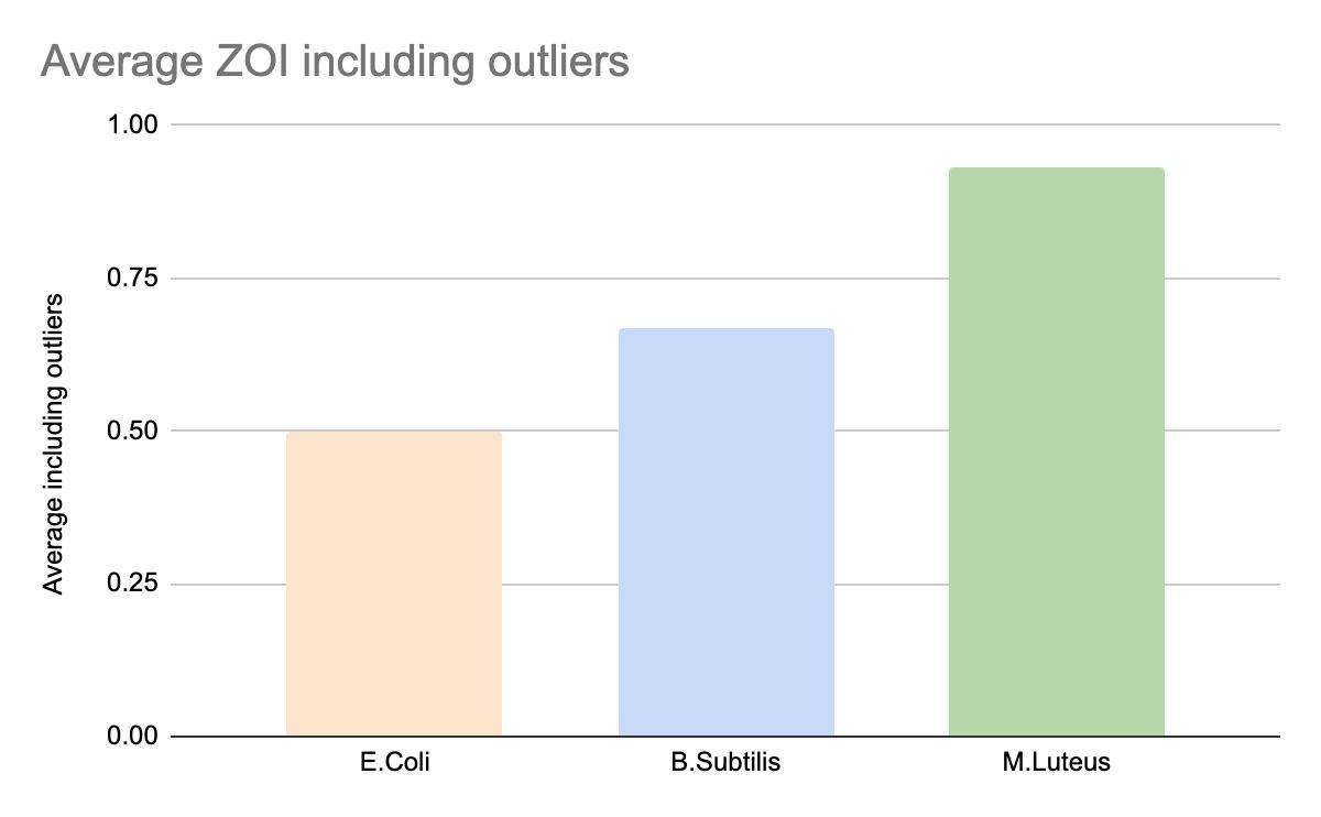
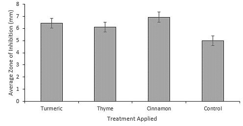
Comparing the antifungal activity of edible essential oils against Saccharomyces cerevisiae

Hooria Malik, Blacktown Girls High School

Thisresearch evaluates theantifungal efficacy of turmeric, thyme, and cinnamon oils against Saccharomyces cerevisiae to determine their suitability as natural food preservatives. All tested oils demonstrated antifungal properties, but there were no significant differences between them, potentially dueto study limitations like small sample size. Thefindings support further research into these oils as potential natural food preservatives, necessitating more extensive studies considering their overall impact on food properties.

199 – 211

The opportunity for modern uses of indigenous and aboriginal medical practices

Amy Mann, Turramurra High School

The research explores the potential integration of indigenous medical practices into modern medicine,focusing specificallyon the antimicrobialeffectivenessofthe Dodonaeaviscosa purpurea, a subspecies used in traditional healing. This subspecies showed minimal antimicrobial effect on the tested bacteria. The research highlights the potential for certain indigenous practices and other subspecies, like Dodonaea viscosa angustifolia, to contribute to modern medicine, particularly in providing antimicrobial treatments.

212

– 226

Naturally occurring sunscreen: An investigation into the effectiveness of squid ink melanin as a UV blocker, compared to current physical and synthetic UV protectors

Thestudy investigates thepotential of squid ink-derived melanin as a UV protectant. Thestudy concluded that there was nosignificant correlation between R-value changes and melanin’s or nanomelanin’sefficacy in UV protection. Results highlighted potential avenues for future research, including in vivo research on melanin’s real-world applications in UV protection, especially as nanoparticles, and for its possible cosmetic advantages.

227 – 237

The effect of Artemisia absinthium on Staphylococcus aureus by comparing the zone of inhibition between 10µl and 15µl of Artemisia absinthium

Sherab Pelmo, Armidale Secondary College

This study evaluates Artemisia absinthium oil’s antimicrobial impact on Staphylococcus aureus at different concentrations. A 15 µl concentration of A. Absinthium oil more effectively inhibited S aureus growth, denaturing more bacterial proteins. This study supports the potential use of A Absinthium as an alternative antimicrobial agent in the face of rising antibiotic resistance, underlining the need for further exploration and product development.

238 – 251

Antifungal effect of Camelus dromedarius urine on fungal colonies –namely Saccharomyces cerevisiae

Hannah Rose, Gosford High School

ThereportexploreswhetherCamelusdromedarius(camel)urineinhibitsthefungusSaccharomyces cerevisiae, compared to the standard antifungal Fluconazole. While camel urine showed antifungal properties,thedifferenceineffectivenesscomparedtoFluconazolewasnotstatisticallysignificant. The study indicates potential for Camelus dromedarius urine as an antifungal agent, suggesting avenues for future research and potential development of alternative antifungal treatments.

252 – 276

The effects of probiotics on Saccharomyces cerevisiae growth

Tilly Rose, Crookwell High School

To determine theimpact of specific probiotics on thegrowth of Saccharomyces cerevisiae, a type of yeast. The growth of S. cerevisiae significantly increased when inoculated with probiotics like Lacticaseibacillus rhamnosus and Streptococcus thermophilus. These preliminary results suggest a beneficial relationship between certain probiotics and yeast, indicating potential applications in thehealth and food industries. However,further research isneeded to confirm these findings and understand the underlying mechanisms.

277 – 290

Influenceof contrasting versuscomplementarycolour conditionson short-term recall

Shaan Singh, Coffs Harbour Senior College

This study seeks to investigate whether contrasting or complementary colour conditions affect short-term memory recall of words in a digital format. Thestudy found negligible influence of both contrasting and complementary colours on short-term word recall. These results suggest that other sensory factors or revised methodologies should be explored to understand memory’s complexities and guide educational and design practices related to learning tools.

IN THIS EDITION

291 – 306

The purpose behind dreaming

Tiffany Tanasale, Northmead Creative and Performing Arts High School

This study explores a variety of theories and personal contexts to discern any consistent purpose behind human dreams. Analysis shows that dreams do not serve a single purpose but are a subjective interplay of neurobiological processes, subconscious longings, and simulated social scenarios based on individual contexts. Understanding the multifaceted nature of dreams opens avenues for self-discovery,personal development, and societal advancement,encouraging further interdisciplinary research in this mystifying aspect of human cognition.

307 – 316

Linking traitsof the five factor model of personality toclinical and subclinical levels of substance use

Vincent Tannos, James Ruse Agricultural High School

Theresearch explores theconnection between traits identified in theFive-Factor Model of personality (FFM) and clinical and subclinical substance use levels. Subclinical substance use correlates positively with neuroticism and negatively with conscientiousness, agreeableness, and extraversion, aligning with patterns seen in diagnosed Substance Use Disorders (SUDs). Identifying these personality profiles related to substance usecan aid clinicians in early diagnosis and intervention strategies for SUDs, potentially preventing severe progressions.

317 – 329

Cytotoxicity of varying Doxorubicin drug concentration on the HT1080 cancer cell line

Secondary College

The paper investigates the relationship between varying concentrations of Doxorubicin and its ability to reduce cell viability in HT1080 cancer cells. Higher Doxorubicin concentration significantly decreased cell viability, establishing a n inversely proportional relationship between drug concentration and cell survival These insights reinforce the use of Doxorubicin in chemotherapy, highlighting theimportance of concentration in maximising therapeutic efficacy against fibrosarcoma.

IN THIS EDITION

330 – 349

Accelerated aging: The effects of vitamin E and vitamin D3 on telomerase activity in MCF-7 breast cancer cells

Marieta Van der Merwe, Menai High School

Theresearch investigates theinfluence of vitamin E and D3 on telomerase activity, which has implications for cellular aging and cancer Vitamin D3 shows inhibitory effects on telomerase, but not significantly, while vitamin Eexhibits a moresubstantial and significant relationship, suggesting potential roles in cancer therapy. The study highlights potential therapeutic roles for vitamins in cancer treatment and the necessity of further research to determine optimal concentrations and combinations with possible broader health and economic benefits.

350 – 361

Systematic review and meta-analysis of acetaminophen dosedependent interactions between oxidative stress and cerebral edema during neurodegeneration

Jasmine Virk, Ryde Secondary College

This report explored the interactions between varying doses of acetaminophen, oxidative stress, and possible cerebral edema in the context of neurodegeneration. Acetaminophen interactions were found to bedose-dependent, suggesting different mechanisms of action within therapeutic and toxic ranges. Thereview calls for clinical trials into acetaminophen’s neuro-protective effects at low doses and its potential in treating neurodegenerative conditions.

362 – 384

Chemotherapy vs immunotherapy in the treatment of non-small cell lung cancer

Geoffrey Yang, James Ruse Agricultural High School

The research compared the effectiveness of chemotherapy and immunotherapy in treating Non-Small Cell Lung Cancer (NSCLC). Immunotherapy showed more favourable results than chemotherapy in overall survival, progression-free survival, and adverse effects, suggesting it should be considered over chemotherapy for NSCLC treatment. The study highlights the necessity for continued research into more personalised treatment options and dosages, particularly considering immunotherapy’s demonstrated benefits in patients’ survival and quality of life.

IN THIS EDITION

385 – 402

Predicting P-glycoprotein inhibition using a message passing graph neural network

Kyle Zhang, James Ruse Agricultural High School

This study evaluated a graph neural network’saccuracy in predicting P-glycoprotein (P-gp) inhibition in new molecules. The model was trained using a dataset of P-gp inhibition and fine-tuned through hyperparameter optimisation. The model achieved superior predictive accuracy (AUC score of 0.946) compared to traditional fingerprinting methods. The approach promises to enhance drug discovery processes, offering a more efficient, cost-effective method than existing assays.

403 – 422

Hyaline mucus allorecognition in myxomycete Physarum polycephalum as a product of dissimilar metabolic composition of extracellular slime tracks

Nick Apalis, Gosford High School

This study examines if nutrient variations affect allorecognition in Physarum polycephalum slime moulds through themetabolic composition of their slime tracks. No significant allorecognition difference in slime tracks of different metabolic compositions were found, but findings were limited by biases and small sample size. This study contributes to understanding the effects of metabolic factors on allorecognition in microorganisms.

423 – 438

Investigating the co-selection of heavy-metal and antibiotic resistance in E. coli

Darren Bian, James Ruse Agricultural High School

Theresearch investigates theco-selection of heavy-metal and antibiotic resistance in E. coli, a concern dueto its implications on global health. Examination of two studies revealed a significant increase in antibiotic resistance in bacteria from heavy-metal spiked environments. Thestudy demonstrates theneed for strategies to mitigate heavy-metal contamination and advances in alternative therapeutics, such as bacteriophages, to combat the growing crisis of antibiotic resistance spurred by environmental factors like heavy-metal pollution.

IN THIS EDITION

439 – 458

Sodium chloride and food product preservation

Philippa Day, Turramurra High School

Theresearch investigates how varying concentrations of sodium chloride influence thespoilage rate of food products, specifically complex carbohydrates. Higher sodium chloride concentrations significantly slow food spoilage, confirmed by a statistical analysis comparing different concentration levels. The study reinforces the use of sodium chloride in food preservation, providing a scientific basis for its effectiveness in extending the shelf life of food products.

459 – 470

The effect of available nutrients on duckweed biomass production

Isabella Drake,

Thestudy explores how nutrient availability influences Lemna minor (duckweed) biomass accumulation. Nutrient-rich environments significantly enhance L. minor’s growth, implicating water quality management in habitats where duckweed overgrowth poses ecological threats. Theresults suggest duckweed’s potential role in bioremediation efforts for nutrient-laden waters, emphasising the need for controlled nutrient runoff into freshwater ecosystems.

471 – 487

Microplastics, anything but a small problem: An investigation into how different sizes of Australia’s most common waterway microplastic, polyethylene, effects Daphnia magna’s physiological functions

Jessica Jones, Menai High School

This research explores the impact of different microplastic sizes on the physiological functions of Daphnia Magna.Smaller microplastics (425–500 um) significantly affected Daphnia’s physiology, but nosize showed a statistically significant impact on heart rate. Theresults emphasise the need for extensive research on microplastic impacts, particularly considering their potential for bioaccumulation and broader ecological and human health consequences.

IN THIS EDITION

488 – 516

Demonstrating a climatic extinction catalyst through a meta-analysis of Neanderthal population distribution

Abigail Kogan, Gosford High School

The research investigates how ancient climatic shifts affected Neanderthal extinction by examining their migration patterns. Neanderthal’s migrated southwards during glaciations and northward in interglacial periods, showing climate sensitivity. This research offers insights into current and future human vulnerabilities. It underscores the importance of climate change awareness and proactiveness in preserving human societies, drawing direct parallels with prehistoric extinction events.

517 – 528

The green-reality of biodegradable sanitary napkins: how the presence of pH affects the rate of degradability of biodegradable plastics within the lining of sanitary napkins

Simitri Kumar, Blacktown Girls High School

This report assesses the impact of pH molarity on the degradation rate of biodegradable plastics in sanitary napkins. The observed trends between pH molarity and degradation rate were not statistically significant. The findings emphasise the need for further research exploring other environmental and compositional factors influencing biodegradable materials’ degradation, informing the future design of sustainable hygiene products.

529 – 540

Allelopathic effect of Lavandula species on the germination and development of Tagetes sp.

Brooke Lawson, Lambton High School

This research delves into understanding the allelopathic impact of different Lavandula species on the germination and early growth stages of Tagetes sp. by studying the inhibitory effects of their leaf extracts. There were marked differences in allelopathy among the Lavandula species, with L. dentata showing the strongest inhibitory effect. The findings suggest potential agricultural applications for certain Lavandula species, especially L. dentata, as natural herbicides, providing an eco-friendly alternative to chemical options.

IN THIS EDITION

541 – 558

Evaluation of the impact of major human activities on the habitat suitability of coastal freshwater forested wetlands as a species rich ecosystem for waterbirds

Emelia Naumov, Coffs Harbour Senior College

The study evaluates the effect of human activities on freshwater forested wetlands for waterbirds. Agriculture, mining and urbanisation were found to negatively affect habitat suitability, reducing tree and waterbird diversity.Thefindings reinforce theneed for conservation efforts and policies to protect wetland ecosystems from human encroachment, ensuring the preservation of biodiversity and essential natural processes.

559 – 572

What is the effect of the growth of ‘Nannochloropsis’ when exposed to urea and ammonium phosphate fertilisers on dissolved oxygen content in water?

Chandni Premkumar, Blacktown Girls High School

Thestudy examines theinfluence of urea a nd ammonium phosphate fertilisers on thegrowth of Nannochloropsis and dissolved oxygen levels in water These fertilisers were found to boost Nannochloropsis growth, increasing algal biomass and significantly reducing dissolved oxygen. These findings underline theenvironmental implications of fertiliser use,particularly concerning the risk of oxygen depletion in water bodies due to excessive algal growth.

573 – 587

Comparing theefficiencyof plant xylem structureswithin angiosperm and gymnosperm wood in filtering biological contaminants in water

Arsh Sharma, Girraween High School

The research probes the effectiveness of xylem tissues in angiosperms and gymnosperms for water purification by eliminating biological pollutants. A significant contrast was discovered in thecolony-forming units (CFU) between thetwo plant types, with gymnosperm filters restraining microbial contaminants more effectively than angiosperm filters. Theefficiency of gymnosperm xylem structures in water filtration suggests a potential application in low-cost, sustainable purification methods, particularly in developing regions.

IN THIS EDITION

588 – 596

The accuracyof DFT in predicting thecollective movement of fruit flies (Drosophila melanogaster) in response to a heat stimulus

Bhargav Suresh, Cherrybrook Technology High School

The study aimed toevaluateclassical Density Functional Theory (DFT) approximations in predicting thecollective movement of fruit flies in response to a heat. Thestudy demonstrated that adjusted DFT accurately predicts thecollective movements of fruit flies, particularly in response to a heat stimulus. These results emphasise DFT’s potential in modelling and forecasting collective movements in many-body systems beyond traditional applications in physics and chemistry, extending its applicability to biological entities.

597 – 608

The potential of prickly pear cactus for biohydrogen production: An investigation into the effect of temperature on dark fermentative hydrogen production using Escherichia coli k12 with Opuntia spp. as a substrate

Anita Thivakon, Inverell High School

This study explores Opuntia spp. as a substrate for biohydrogen production and temperature effects. Optimal hydrogen production was achieved at 40°C and 25°C, showing temperaturedependent variation. The research points to Opuntia spp’s potential in sustainable hydrogen production, underlining the importance of temperature in fermentation efficacy

609 – 619

Influenceof elevation on Basidiomycota fungi distribution in New England wet sclerophyll forests

Waugh, Armidale Secondary College

ThisstudyexaminesthedistributionpatternsofBasidiomycotafungiinrelationtovaryingelevations within New England wet sclerophyll forests. Basidiomycota fungi show a non-homogeneous distribution, with higher abundances at increased elevations, although species diversity does not correlate with elevation changes. The evident rich fungal diversity demonstrates the ecological importance of these forests, suggesting a need for conservation efforts and understanding the ecosystems’ resilience to environmental stresses.

IN THIS EDITION

620 – 634

Time dynamics of chemical gardens

Jonathan Allen, Lambton High School

The study aims toexamine the vertical growth rateof copper (II) and magnesium (II) salt precipitates in sodium silicate chemical gardens and to understand the relationship between the growth and theproperties of thesalts used. A statistically significant linear relationship was found between themoles of Cu2+ and Mg2+ and theheight of their respective precipitate tubes for thefirst 300 seconds of growth. Thefindings provide a fundamental understanding of thegrowth dynamics in chemical gardens, paving theway for further research into theself-assembly and microstructure of precipitates in chemical systems.

635 – 649

Analysing the relationship between the stellar metallicity of host-stars and insolation flux of the planetary body

This paper explores whether a relationship exists between the stellar metallicity of host stars and theinsolation flux on planets, parameters relevant to thehabitability of exoplanets. While a statisticallysignificant relationshipwas found, thecorrelation is weak, suggesting that other factors may also influence planetary habitability conditions. These findings prompt more comprehensive studies, potentially considering atmospheric compositions, and highlight the importance of new technologies in the search for habitable exoplanets.

650 – 678

A novel mathematical model of the boomerang flight aerodynamics

Hoang

This study sought to create and assess a new mathematical model to predict the trajectories of a returning boomerang accurately. Thenew model showed promise in simulating real-world boomerang flight patternsbut required refinements for accuracyin predicting flights under varying conditions. Thefindings contribute to theunderstanding of boomerang aerodynamics and have practical applications in sports and engineering, thus acknowledging Aboriginal contributions to science.

IN THIS EDITION

679 – 688

Theefficiencyof electrocatalysts in water electrolysis in reference to first ionisation energy

Toby Downes, Armidale Secondary College

Theresearch aims to discern therelationship between thefirst ionisation energy of an electrocatalyst and its efficiency, as indicated by overpotential values during water electrolysis. While statistical evidence supports a significant link between a catalyst’s first ionisation energy and its overpotential, the correlation is not strong, varying with the type of electrolyte used. The results contribute foundational knowledge for enhancing electrocatalyst selection in clean hydrogen production, potentially advancing eco-friendly technology and industrial applications.

689 – 702

Exploring ricochet behaviour in spherical projectiles on water targets

Timothy Harrison, Lambton High School

Thestudy investigates how theangle of attack influences thericochet behaviour of elastic spheres using water targets. A NERF Rival Kronos XVIII-500 Blaster was used to project rounds at a water-filled plastic tank, testing various angles of attack. A significant linear relationship exists between theangle of attack and ricochet behaviour,with specific angles where ricochet ismost prevalent and a peak in cavity depth at a 38° attack angle. These insights emphasise theutility of NERF Rival Blasters as safe, educational tools for studying ricochet dynamics, providing practical understanding and engagement for high school students.

703 – 716

Limitations of special relativity for an understanding of causality around spacetime singularities

Adam Inger, Barrenjoey High School

This paper explores the impact of Special Relativity on understanding causality, particularly in spacetime singularities and scenarios involving high velocities. The study showed causality is preserved under Special Relativity, though event sequences vary. In contrast, exceeding light speed results in causality inconsistencies and retro causality. This confirms Special Relativity’s role in defining causality limits, but calls for more detailed research due to the study’s simplified approach.

IN THIS EDITION

717 – 747

Limitations in superheavy element synthesis

The paper discusses the challenges and future prospects in synthesising superheavy elements beyond thecurrent 118 known elements. Advances in experimental techniques and equipment may soon overcome existing synthesis barriers, with potential breakthroughs anticipated in the next decade. These advancements could significantly broaden our understanding of atomic structures and facilitate the synthesis of previously unknown elements.

748 – 759

The effects of diameter in synchronised metronomic systems

Prabhjas Sandhu, Ryde Secondary College

To explore how thediameter of PVC pipes influences thesynchronisation time of coupled metronomes. Larger diameters of PVC pipes facilitate quicker synchronisation of metronomes, though anti-phase synchronisation remains unaffected by thediameter These findings enhance understanding of emergent phenomena and collective behaviour,potentially influencing complex systems’ design and network science, especially where synchronisation is crucial.

760 – 778

The relationship between aerodynamic properties and the leading-edge radius of an aerofoil

Jayden Sandison, Illawarra Sports High School

Thisresearch examines how changes in theleading-edge radius of an aerofoil influence its aerodynamic performance. Modifications in theleading-edge radius directly affected theaerofoil’s lift-to-drag ratio, with smaller radii yielding more favourable aerodynamic properties. These insights into aerofoil design parameters may inform more efficient designs in various aerospace and automotive applications, potentially enhancing performance and sustainability.

IN THIS EDITION

779 – 790

Comparing the effectiveness of NiAsOx-, MnAsOx-, and ZnAsOxloaded mesoporous silica nanoparticles at decreasing the viability of human liver cell cultures in vitro

Jeremy Stephens, Normanhurst Boys High School

Thisstudysought toevaluatetheeffectivenessof threedifferent arsenictrioxide(ATO)loaded mesoporous silica nanoparticles on human liver cancer cell viability. The NiAsOx complex was more effective, with faster ATO release correlating with greater effectiveness, though not statistically significant.Thisindicatespotential for nanoparticle-assisted drug deliveryfor cancer therapy,but necessitates further research for enhanced treatment efficacy.

791 – 808

Theeffect of fin sweep angleon a model rocket’s flight

Thestudy evaluates how altering thesweep angleof fins on a model rocket influences its maximum altitude, or apogee, during flight. A significant correlation exists between thefin sweep angle and therocket’s apogee, with increased angles resulting in higher flight, supported by statistical data showing a high correlation. The research suggests practical applications in enhancing rocket design efficiency, potentially informing more cost-effective aerospace engineering practices.

809 – 815

Effectivenessof natural language processing in identification of components of secondary school argumentative essays

The study aimed to evaluate natural language processing (NLP) in identifying various elements within HSC English argumentative essays. The program demonstrated a mean accuracy level of 64% in identifying essay components, coupled with a notably low error rate of 2.3%, indicating that its current state of accuracy in component identification aligns only moderately with the standard expectations. Theresults suggest NLP’s potential in providing efficient, targeted feedback on student essays if their accuracy can be improved.

IN THIS EDITION

816 – 829

Enhancing aircraft bending stresscapabilities and fuel efficiencywith WrapToR composite trusses

Baden Manson, Ulladulla High School

The study investigates whether implementing a WrapToR composite truss within an aircraft’s structure enhances its bending stress capabilities and subsequently improves fuel efficiency. While results varied, the study found indications suggesting improvements from incorporating a WrapToR composite truss in aircraft wings. This research suggests potential advancements in aerospace engineering and design, pointing towards the use of composite trusses as a viable solution for enhancing aircraft performance and operational cost-effectiveness.

830 – 845

Theeffect the addition of a 3-qubit bit fliperror correction code hason the fidelityof a quantum computation

Liam Mitchell, Grafton High School

Thestudy assessed how a 3-qubit bit flip error correction code influences thefidelity of quantum computations Fidelitylevelsweremeasuredusingquantumerrorcorrection,comparingresultswith and without the 3-qubit code. Implementing the 3-qubit code significantly improved computation fidelity, highlighting its effectiveness in managing quantum noise and errors. Thisadvancement bolsters thereliability of quantum computing, contributing to its practical application in complex computations and simulations.

846 – 858

DFT method defiesconventional wisdom, accuratelycalculates corannulene enthalpy

Finley Wallace, Peel High School

This study sought to evaluate different Density Functional Theory (DFT) methods in predicting theenthalpy of transition of corannulene from a bowl-up to a bowl-down orientation. The M06-L functional showed high accuracy (0.4 kj mol-1 error), surpassing others despite not being specialised for corannulene. These findings challenge theconventional understanding of DFT methods and suggest that theM06-L functional could bemore widely applicable than previously thought and may lead to significant advancements in computational chemistry

Introduction to invited paper Evaluating Science Extension

Olivia Clarkson completed Science Extension as part of her HSC studies in 2019.Last year,Olivia completed her Bachelor of Science (Advanced) studies at the Universityof Newcastle.Olivia took thethird-year SCIE3500 Research Integrated Learning courseas part of her program. The Research Integrated Learning course – like Science Extension – allows students to pursue an individual research project. Interestingly, Olivia used the opportunity to undertake an evaluation of the Science Extension course, and the following paper is based on Olivia’s evaluation. This year, Olivia is enrolled in the University’s Honours program year and will continue researching the impact of Science Extension on science education in NSW schools.

Olivia’s research supervisors for this paper are Dr Bonnie McBain and Dr Liam Phelan, both from the School of Environmental and Life Sciences at the University of Newcastle. Drs McBain and Phelan have research interests in complexity science and science education. Drs McBain and Phelan supported Olivia in framing theresearch question, discussing appropriate evaluation methodologies, and providing guidance through the research and writing processes.Since2017,DrsMcBain and Phelan have led the transformation of science education at the University. The University’s ambition is to produce science graduates (i) who are strong in their disciplinary knowledge and skills, (ii) who are also able to work with others across disciplines in order to engage effectively with contemporary, wicked problems facing societies such as climate change, the obesity epidemic and the housing crisis, and (iii) who are ready to apply their science way of thinking in multiple contexts – in the world of professional science work and beyond.

We are grateful to Dr Sham Nair, Science Advisor 7-12,and Mr ChrisBormann,ScienceCurriculum Officer,from theNewSouth WalesDepartment of Education, for ongoing conversations about the future of science education.

Evaluating Science Extension

Perspectives from the literature, teachers, students and mentors

Olivia Clarkson

Third-year student, Bachelor of Science (Advanced), University of Newcastle

ScienceExtension is a Higher School Certificate(HSC) coursein NewSouth Wales.Thecoursecomprises a year-long individual student project,followed by an HSC exam. The course focuses on developing students’ science skills through individual projects.In thisstudy, I evaluatethequalityof scienceeducation in ScienceExtension.ScienceExtension wasfirst offered in 2017 and evaluation nowistimely I began bydrawing on thescientificliteraturetoidentifytwothemes (pedagogy and science skills) and a range of criteria to identify high-quality science education. On that basis, I then reviewed Department of Education documentation to evaluate the intended learning outcomes of the current Science Extension syllabusand curriculum reform goals.Lastly, I analysed thirty-onetranscripts from interviews with students, teachers and mentors about their experiences with Science Extension. This analysis evaluated if the experience of participants aligned with high-qualityscienceeducation and theintended learning outcomes. Through thisprocess,additional themesemerged from transcripts:scientific practice, engagement and limitations.

Feedback from students, teachers and mentors showed Science Extension implemented high-qualityproject-based learning,washighlyrelevant tostudents and their individual passion for particular scientifictopicsand allowed students to effectively learn statistics in a collaborative environment that replicated the wayscienceisdone in thereal world.Theevaluation findsthat ScienceExtension isgrounded in,and offersstudents, a high-qualityscienceeducation.Expanded accesstomentorsand scientificpublicationsisidentified as a further opportunity to support students’ learning.

Keywords: pedagogy, high quality science education, student-centred learning, science skills.

Introduction

The contemporary world is characterised by rapid n.d.; National ScienceTeaching Association,2011). global change,reprioritising theneed for scientific Theskillsinvolved in high-qualitysciencesuch as focuson big societal challengessuch asartificial critical thinking,problem-solving,collaboration, intelligence (AI) and machine learning, climate scientific literacy, science communication, change, health and pandemics, alternative energy, and systems thinking, are essential for future sustainability and food security (United Nations, generations to learn to contribute to and engage

with big challenges (Kubisch et al., 2022; National Science Teaching Association, 2011). Beyond disciplinarylearning,high-qualityscienceeducation isabout decision-making,communication and critical thinking to solve problems (Kubisch et al., 2022; Osborne, 2006).

• Secondary schools can provide students the opportunity to learn needed high-quality science skills. High-quality scienceeducation includes, but is not limited to:

• Integrated curriculum – teaching multidisciplinary and interdisciplinary science, rather than individual sciences only (Wang et al., 2020)

• Scientific inquiry–encourage evidence-based practice and investigation (Rufell, 2022; Alberts, 2022)

• Scientific literacy– the ability to distinguish high-quality science, preventing the spread of misinformation and misunderstandings (Kubisch et al., 2022; Rufell, 2022)

• Collaboration in problem-solving – between students, and collaboration with scientists (Wang et al., 2020; Shanahan & Bechtel, 2019).

There is consensus among students, teachers, researchers and the Department of Education that science teaching and learning opportunities should berelevant (Masters,2020; Bidarra & Rusman,2017; Stuckey et al 2013; Newton,1988).However,theterm ‘relevant’ has been a point of discussion in science education for manyyears(Newton,1988).‘Relevant’ is a broad term that is contested.

‘Relevant’ in science education can apply to course content, learning opportunities, and pedagogy. It can be the nexus between school courses, tertiary education and future work (Masters, 2020; Busch, 2005).Learning should alsoberelevant in termsof both student and societal contexts – this may direct student interest tohealth or environmental-based topics in science, for instance (Stuckeyet al. 2013).

Literature review – what is relevant to high-quality science education?

This evaluation begins with a review of the scholarly literature on science education. From the review of theliterature, I identifyseveral criteria for highqualityscienceeducation,categorised intotwo themes – pedagogy and science skills. These are discussed below.

Pedagogy – active, self-directed, problem-based, and collaborative learning.

A best practice pedagogical approach to science teaching includes instructional design that is both flexibleand can providesupport for students todeveloptheir learning pathwaysand specific learning objectives(Bidarra & Rusman,2017 ).It is student-centred learning.

Oneof theprimarygoalsof thispedagogical approach is to engage students in active learning to encourage student engagement. It encourages engagement through ‘meaningful learning activities’ which can increaseboth short-term and long-term retention of information (Ruhl et al. ,1987; Mastascusa et al 2011; Prince, 2004).

Active learning can encompass many different activities.For example,Overton & Johnson (2016) presented some sample student activities:

• Students interpreting the ‘core concepts’, or the syllabus and learning outcomes of lessons themselves– self-directed learning.

• Providing problems and learning scenarios that require reflection and reviewing of students’ knowledge via practical application of knowledge–problem-based learning through application of curriculum content.

• Undertaking peer review to explore alternative learning perspectives and enhance student understanding –collaborative learning.

Activelearning integrated with problem-based learning enables students to develop their own pathwaysand goals.Problem-based learning in a real-world setting or with relevant scenarios(Overton & Johnson, 2016), can be based on student’sindividual learning goals and levels, allowing students to learn through problem-solving (Hattie,2013; Lovenset al. , 2016).Thistypicallyinvolvesstudentsin learning partnerships –working in small groups with peers.

Problem-based learning promotesgreater academic success and achievement when students work collaboratively (e.g. in small groups), than if they work individually (Norman & Schmidt, 2000; Ajai et al. ,2013).Thistypeof problem-based learning also assists students in developing transferrable skills, such as critical thinking and teamwork, applicable to future education and employment (Overton & Johnson, 2016; Ajai et al., 2013).

Collaboration iscommon in project-based learning activities (Manlove et al., 2006). One of the methods used to facilitate collaboration in science is peer assessment and peer feedback and review–students review, comment, assess and suggest improvements to the work of other students (Mora et al., 2020). As students practice peer review and assessment, the qualityof their work improvesover time(Rotsaert et al., 2018).

Self-directed learning requiresstudentstoset individual learning goals, regulate and plan their learning, adjust their learning strategies, and being abletoreflect on their learning (Brandt,2020).Selfdirected learning isessential for effectiveproblembased learning and completion of tasks(HmeloSilver, 2004).

Science skills – statistics, science communication, scientific method; critical and creative thinking.

TheOfficeof theChief Scientist (2015) outlineskey skills to be developed in undergraduate (tertiary) science courses and thus is relevant to Science Extension to prepare HSC students for continuing their science studies at university. These include transferrable skills such as communication, time management, complex problem solving, creativity, critical thinking,and discipline-specificskillssuch asthescientificmethod,evidence-based practice– literature review, and numerical competency, such as statistics.

Critical thinking is an essential skill for developing scientificliteracy(Manassero-Mas& VazquezAlonso, 2022). Critical thinking links heavily with the abilitytorationaliseand developscientificreasoning –both are essential for students when engaging in research projects and reading research papers (Dowd et al.,2018).It isa keyskill that linksnot only to research projects and papers, but also enables students to link concepts together across different research and different disciplines. Bridging across different disciplines allows students to engage in multidisciplinary and interdisciplinary science, thereforeengaging in an essential element of highqualitysciencepractice(Wang et al.,2020; Dowd et al. 2018).

The ability to think critically enables students to engagein scientificinquiry,and thusthescientific method (Forawi,2016).Unlikesimplylearning about science, practicing science and implementing the scientificmethod enablesstudentstoexperiencethe linksbetween scientifictheory,experimental design and data, alongside learning how to present and concludetheir own investigations(Hodson,2014).

Ultimately,engaging with thescientificmethod teachesstudentshowtoask effectivequestions, which isthebasisof science(Hodson,2014; Vale, 2013).

Statistical literacy is important when absorbing research papers to judge the reliability and accuracy of anyfindingsin thepaper,essential for developing scientificliteracy(Ritchie,2020).Statisticsenables significancetobetested and thusisan important contributor toscientificknowledge(Horton & Hardin, 2015).Learning statisticseffectivelycan lower math anxiety and increase student performance in the sciences (Wilson, 2013).

The ability to communicate science and abstract conceptsisanessential element of science(MercerMapstone& Kuchel,2015).Scientistsneed tobeableto effectivelycommunicatetheir findingsand research to unfamiliar or uninformed audiences (Dahlstrom, 2014).Effectivesciencecommunication tononexpert audiences or across disciplines reduces the sharing of misinformation and misunderstandings (Van Bavel et al., 2020). Examples of this were seen during theCOVID-19 pandemic,whereineffective science communication increased the popularity of conspiracy theories, misinformation and fake news (Van Bavel et al., 2020; Fraser et al., 2021).

In summary,a reviewof theliteratureidentified several criteria which constitutehigh-qualityscience education, categorised into two themes – pedagogy and science skills:

1.Pedagogy

• Problem-based learning

• Active learning

• Student-centred learning

• Collaboration

• Self-directed learning

2.Science skills

• Science communication

• Critical thinking

• Creativity

• Statistical analysis

Research aims

This study aims to provide an evaluation of the Science Extension course grounded in relevant

literature and drawing on (i) Department of Education documentation, and (ii) students’, teachers’ and mentors’ experiences engaging in the course in recent years.

Research methodology

Evaluating Science Extension was based on criteria that emerged in the preceding literature review. To review the literature and identify emergent criteria and themes I used NVivo software. As criteria arose, they were coded into NVivo.

These criteria were used to analyse (i) Department of Education documentation and (ii) transcripts of interviews with students, teachers and mentors.

Department of Education Documentation

Two documents were received from the Department of Education–1) a curriculum review (NESA, 2020) and 2) the course syllabus (NSW Education Standards Authority,2017 ).Thecurriculum reviewdocument outlined skills that were to be introduced in the new curriculum. The Science Extension syllabus provided the intended learning outcomes of the course. The syllabus was also used as a comparative tool for curriculum evaluation after transcript analysis and theme coding occurred.

Interview Transcript Analysis

Interview transcripts were analysed to identify the experiences of students, teachers and mentors which aligned with criteria for high-qualitypedagogy and science skills. Additional ad hoc themes became obvious as transcripts were analysed. These codes were added to NVivo as they emerged and were iterativelyrefined asfurther analysiswasundertaken.

Interviewtranscriptsfrom twenty-nineseparate interviews with Science Extension students, teachers, or external student mentors were received from the Department of Education.Fifty-two per cent of transcripts were students, 34% were teachers of Science Extension, and 14% wereexternal mentors.

Random subsampling was used to determine the order in which to analyse transcripts. Each transcript was prescribed a number. A random number generator was used to choose a subset of ten initial transcripts from students, teachers and mentors. The random selection process was repeated until all transcripts were coded in NVivo. This minimised any bias associated with the order interviews were undertaken.

Introducing the Science Extension curriculum

The following information is sourced from the Science Extension syllabus (NSW Education Standards Authority, 2017 ).

Science Extension is structured around students designing and completing a year-long individual research project – they choose the subject, and experimental methods, complete data analysis and summarise conclusions in a research paper. This is followed by an HSC exam that tests the skills students should have developed while undertaking their projects, such as statistical literacy and critical thinking.

There are four modules in the Science Extension curriculum, each focusing on a different element of scienceskillsand pedagogy Module 1 focuseson thetheories(such asinduction,falsification and bias) and ethics in science. Module 2 focuses on students’ research proposals and project design. Module 3 focuses on statistical analysis and interpretation of results. Module 4 focuses on the structure and function of students’ final research report.

One of the overall goals of Science Extension is to provide a foundation for students with an interest in STEM to be able to “pursue further study in Science, Technology, Engineering or Mathematics (STEM) based courses offered at the tertiary level, and to engage in new and emerging industries.”

To reform the New South Wales science curriculum toengagewith high-qualityscienceeducation,a curriculum reviewcommenced in 2018 (Masters, 2020; NSW Education StandardsAuthority,2021).

In 2020,Geoff Mastersconducted a K-12 curriculum reviewfor educational reform and outlined a 10-year plan for all curriculum changes.

Changes to curriculum aim to produce contemporary, high-qualityeducational practicebydecluttering syllabi to allow students opportunities to engage and transfer learnt skills across other courses; to provide studentsopportunitiestoengagein problem-based learning and projects; and to provide learning opportunities for students that are technologically and globally up to date.

StageSix (year 11 and 12) syllabi arebeing renewed at the time of writing and will be released in 2024 (AIS NSW, 2022; Masters, 2020). The stage syllabi werereviewed between 2017 and 2019.Elementsof the current syllabus will remain in the new syllabus.

Table 1 –Transferrableskills in science(Office of theChief Scientist,2015) and how each skill iscurrently presented in the Science Extension syllabus (NSW Education Standards Authority, 2017)

Transferrable Skill

Communication

Time management

Complex problem solving

Creativity

Critical thinking

Scientific method

Literature review

Statistics

Where skill is present in Science Extension curriculum

Objective SE-6. Objective SE-7. Module 4: The Research Report

The Scientific Research Portfolio Section 1

Module 2: The Scientific Research Proposal

Learning Across the Curriculum

Learning Across the Curriculum

ObjectiveSE-1.ObjectiveSE-3.ObjectiveSE-5.ScienceExtension Stage 6 Syllabus

Objective SE-3. Module 2: The Scientific Research Proposal

Objective SE-4. Module 3: The Data, Evidence and Decisions

Someof thetransferrableskillsidentified bythe Officeof theChief Scientist areembedded in the current Science Extension syllabus in various ways (Table 1, above).

Findings and discussion

Pedagogy

Self-directed learning includesmonitoring individual learning processesand reflectivepractice(Brandt, 2020). For students studying Science Extension, oneof theprimaryplacesself-directed learning is explicitly evident is in their assessment tasks. For example, Student 6 outlines one of their assessment tasks being “a poster and a speech where we had to talk about our background plan for methodology, timeline…” – students individually plan all aspects of their projects.

Self-directed learning and problem-based learning each can alsocentrearound attempting tofind solutionstoreal-world problems(Brandt,2020).This characteristic is evident in student projects as they state that projects “allow you to visualise what’s in the real world, how they implement sciences in the real world, and the impact of those sciences on the real world.” (Student 1).

Due to the nature of the research project, the type of collaboration students engage in does not entirely align with the literature expectation of student collaboration in project-based learning.Specifically,

students do not work in groups to complete their projects. However, students collaborate in other forms - peer reviewand feedback and teacher/ mentor feedback.

Students collaborate via peer discussion: “We become like a team of researchers. I encourage everyone to work and collaborate on each of their projects, so we have a lot of peer discussion.” (Teacher 4). Students will encounter this type of collaboration in tertiary study or employment (Hall et al. ,2018).Teachersarenot experts in each student’s research area,asboth studentsand teachersfind it valuable that students “collaborate with each other when they encounter problems.” (Teacher 7).

Students are also able to collaborate to prepare for exams: “We didn’t collaborate as much with projects, but with thesyllabusitself.”(Student 5).Onestudent recounts their experience of preparing for assessment byfinding papersrelevant tosyllabustopicssuch as paradigm shifts and then engaging in groupdiscussion to practicequestions about the article.

Science Skills

Creativityin sciencecan bedefined astheability of someone to create new and novel ideas (Dehaan, 2009).An application of creativityisproblem-solving. For students studying Science Extension, access to university-level,expensiveequipment isnot always reasonable,nor in budget. A student required access to a carbon dioxide incubator, which would cost

approximately $7000. Instead, the teacher and staff created a DIY carbon incubator, “we bought Kmart containers, sealed them with silicon and drilled a hole through the side to put a carbon dioxide sensor through. We used a soda stream to supply carbon dioxide directly into the container” (Teacher 4).

For both project and exam purposes, students need to be able to apply both creative and critical thinking. For example,studentsarerequired to“extract as much information as you can from [different exam stimuli] rather than…memorising”(Student 8) in the HSC exams.Thisrequires a combination of creative thinking –how can I apply different thought processes tothisstimulusquestion for thebest answer,and critical thinking – joining concepts learnt across the Science Extension course and other science courses. Other critical thinking skills are developed in data collection, for example, “When I found myself list without [knowing] how do I get from this set of data that’s not working to a set of data that does work, it really forced me to make these connections because nooneelse is going to” (Student 12).

Teacher 10 states“Oneof thecoreskillswehope students develop is to be able to critically analyse any information” – including statistics. Connecting, collecting and analysing data – either primary or secondary data is an essential element of Science Extension and the focus of Module 3: The Data, Evidenceand Decisions.Specifically,students typicallyneed tobestatisticallycompetent tofulfil thecourserequirementsand create a supported, evidence-based paper

Statistical competency is important for three reasons.First,manystudent projectsrequire analysis of a lot of data to create meaning with, “It’s data mining and statistical methods are critical. So they learn [statistics], we teach them how to… and help them implement [statistics] in the project” (Mentor 1).Studentswill alsoneed tobestatistically competent for the exam, which results in teachers using “authentic examples for the basis of problems in the statistic module and exercises… that enable students to actually engage with the problems” (Teacher 1).

Learning statisticsbenefitsstudent assessment,but it also provides students the opportunity to learn something that’s “not covered in any other school subject” (Teacher 3), and is typically encountered as a university undergraduate student. For example, Student 14 compared their experiencetotheir father’s, “[dad] was like, oh we learnt this in university, and… I’m doing it now”. Student 3 emphasised this

experience, “being able to use all those statistical tests will give you a leg up in uni no matter what university course you do.”

Interpreting and reporting results (i.e. science communication) is also essential as “there is zero point of doing science if you cannot communicate it to industry partners, the media and your colleagues and peers”(Mentor 1).Being abletowritetheir report “to the standard that would be generally accepted bythescientificcommunity”(Student 2) is a skill students learn and a goal outlined in the Science Extension rationale (NSW Education Standards Authority, 2017 ).

Somestudentsfind it challenging for various reasons, such as the “use of sophisticated language but also going straight to the point” (Student 3). However, despite communication challenges, Student 7 and Student 9 agreethat “scientificreport writing/scientificwriting skillshavebeen useful”in many classes they now study at university.

Each school student “aretheexpert”(Teacher 1) on their topic. They need to be able to “communicate complex topics and abstract theories in simple terms to an otherwise unfamiliar audience” (Student 12).Studentscommunicatetheir knowledgeand ideastotheir teacher –not an expert in everyfield of study, and sometimes students get an opportunity to present their research to either “parents and interested students for the following year” (Teacher 4), or sometimes at the “Young Scientist Awards” (Teacher 7).

Three other themes emerged from the analysis –scientific practice,engagement and challenges.

Scientific Practice

To begin their projects, students decide on topics: “something I could understand, something I was interested in, and then something that had relevant data”(Student 5).Astheycontinueexploring their projects and accessing literature, the challenge is to“narrowdown to a question that wasfeasible” (Student 8).

Students encountered mistakes and failure in various forms.First,thenatureof scientificinquirymeans that experiments will go wrong. The way students attempt to rectify these challenges encourages engagement in thescientificmethod.For example, after encountering mistakes with experimental methods, students were able to “manage fixing errors and trying to do it again just to make sure everything isworking properly”(Student 14) and being ableto

“finesse it andgothrough a fewdifferent trialsto get it to work” (Teacher 7) –it’s a problem solving and revision of their method.

Time management is an essential element of student projects.Student 6 statesthat their first assessment involved “our background plan for methodology, timeline…” Outlining their timeline and goals across the year is essential as students have approximately “an hour of classtime”(Student 15) dedicated totheir projects each week. Timing varies with each project. For example “ theprocessof developing a question took quite a while” (Student 8).

Time management is important for teachers to takenoteof aswell For exampleTeacher 10 states “There is a balance between providing enough time for studentstoproduce a final product, a research report that isquitecomprehensive,and also balancing at the end of the course they need to sit a two-hour onlineexam.”

One of the interesting claims present in the transcripts is that to effectively regulate the timing and structure of the Science Extension course based on their student’s projects, some teachers will “tailor the course depending on student’s projects” (Teacher 7).

Engagement

Engagement was a strong theme in interviews. Engagement comes from the degree of passion studentsshowwhen learning (Groccia,2018).What encouraged students to take the course was that it was an opportunity for students to explore their own passion in science.

Teachers, for instance, have noted that there are many students who “have a deep curiosity for particular areas [of science], a passion they can’t extend in their existing courses” (Teacher 7). With the foundation of Science Extension about an individually focused research project, rather than course content, students have been able to explore areas “beyond school” (Teacher 8).

Unlikeother course-oriented extension courses, such as Mathematics Extension, the ability to curate the course to their individual interests enables students who are not high achievers to study the course. Teachers and students alike stated that the primary indicator of success in Science Extension is not a high grade or to be a high achiever. Rather students must have curiosity and passion for their subject,or a question theywant to answer

The ability of the course to be tailored to each student provided relevance. By exploring their passion in a subject relevant to their context or future career goals, they “get to see how that passion can extrapolate into the real world… as a job or career path…” (Student 1).

Science Extension projects lead to many opportunities for students. The ability to “explore pathways in forensic science that is not possible in anyother subject”(Teacher 8) provided a pathway for a student to study tertiary forensic science. Some students had their projects taken up by teams of researchersat universitiesfor post-graduate study.Other studentssubsequentlystudyunder their [academic] mentor at university due to their project. Science Extension was designed to be a pathway for students to work in or study science, and that pathway is successful for some students (NSW Education Standards Authority, 2017 ).

Challenges

Themain limitationsof ScienceExtension identified are not about the course content or structure, but rather about accessibility. The key opportunity identified through thisevaluation istoincrease accesstomentorsfor student projectsrequiring specificexpertise(not all student projectsrequire them).

Many students don’t have access to specialist mentors in universities. The role of a mentor is to provide support and guidance for each project they oversee. Unlike teachers, who provide essential guidance to every one of their students, “the role of the mentor is more content driven. It’s to provide them with expert knowledge that [teachers] can’t or may not have answers to” (Teacher 6). Through a mentor, students should have access to an expert resource. However, some students doing Science Extension don’t have mentors as “the student’s particular project is just not aligned with that” (Teacher 7). My recommendation is to increase access to mentors through universities in NSW.

Some universities, such as the Universityof Newcastle and the University of Sydney have programs where students can be matched with a mentor that aligns with their research project. Engaging with other universities would enable a wider range of students tofind mentorsthat align with their research focus. This would also increase mentoring opportunities for those in regional areas.

For students with mentors, one of the primary comments was “My mentor had access to [literature] that our school didn’t have.”(Student 5). A literature review is essential for their research project. TheScienceExtension outcomeSE-3 requires studentsto“interrogaterelevant and valid peerreviewed scientificresearch”.However,dueto limited OpenAccess articles, some students resort towebsitesthat “aren’t quitelegal”(Student 3) toaccesstheliteraturerequired for their project. Access to literature is another primary issue that requires fixing for future students.

Conclusion

ScienceExtension implementshigh-qualityscience into the curriculum. Based on the four themes –scienceskills,pedagogy,engagement and scientific practice,ScienceExtension implementshighquality,effective scienceeducation.

Science Extension is not overloaded with course content, leaving room to explore concepts and skills in depth (Masters, 2020). This contrasts with disciplinary secondary science courses. Science Extension course content is centred around individual student projects,i.e. ,problem-based learning.Within problem-based learning,students can engagein high-qualitysciencepedagogy,such asself-directed learning.Studentsdeveloptheir projects, implement appropriate learning strategies, locate appropriate resources, and set their own outcomes and goals (Brandt, 2020). By engaging in problem-based learning and self-directed learning, the syllabus enables students to tailor their learning based on their passion. This is highly effective for student engagement (Groccia, 2018).

Another important element of Science Extension that enablesengagement in high-qualityscience education is collaboration. While each student has their own individual project, students work together tobrainstorm and problem-solveasa team of researchers would. This aligns strongly with the curriculum goal to “prepare students for further academic study” (NSW Education Standards Authority, 2017 ).

Many science skills such as statistics, critical thinking and science communication have supported students in preparing for further academic study. These skills also assist creation of an integrated curriculum (Wang et al., 2020).

The evaluation has found one opportunity to further improve Science Extension: attention to external support such as mentoring programs and increased accesstoscientificdatabaseswill likelybehelpful for students’ learning in Science Extension.

Thefinal evaluation wasbased on positivefeedback from students, teachers and mentors in interview transcripts, overlap between the transcripts and literature, the evaluation criteria, and alignment with the goals of the curriculum documentation. Science Extension – it’s outcomes, objectives, assessment and content –is a highlyeffectiveand high-quality science education.

Further research in this area could include evaluation over a longer period and across all of NSW.

References

AIS NSW. (2023). NSW Curriculum Reform Update. https://www.aisnsw.edu.au/Course%20and%20 Conference%20Materials/21_Timeline%20for%20 Implementation.pdf

Ajai, J T. ,Imoko,B. I. ,O’kwu,E.I.(2013).Comparison of theLearning Effectivenessof Problem-Based Learning (PBL) and Conventional Method of Teaching Algebra.Journal of Education and Practice,4(1),131135. https://core.ac.uk/download/pdf/234633889.pdf

Alberts, B. (2022). Why science education is more important than most scientists think. FEBS Letters, 596(2), 149-159. https://doi.org/10.1002/18733468.14272

Brandt, W. C. (2020). Measuring Student Success Skills:A Reviewof theLiteratureon Self-Directed Learning. https://files.eric.ed.gov/fulltext/ ED607782.pdf

Busch,H.(2005).IsScienceEducation Relevant? Europhysics News, 36(5), 162-167 https://doi. org/10.1051/epn:2005505

Dahlstrom,M.F.(2014).Using narrativesand storytelling to communicate science with nonexpert audiences.PNAS,111,13614-13620.https://doi. org/10.1073/pnas.132064511

Dehaan, R. L. (2009).Teaching creativityand inventive problem solving in science. CBE Life Sciences Education,8(3), 172-181. https://doi.org/10.1187/ cbe.08-12-0081

Dowd, J. E., Thompson, R. J., Schiff, L. J., Reynolds, J. A.(2018).Understanding theComplex Relationship between Critical Thinking and Science Reasoning among Undergraduate Thesis Writers. https://doi. org/10.1187/cbe.17-03-0052

Fraser, N., Brierley, L., Dey, G., Polka, J. K., Palfy, M. ,Nanni,F. ,Coates, J A.(2021).Theevolving response of preprints in the dissemination of COVID-19 research and their impact on thescience communication landscape.PLOS Biology,19(4). https://doi.org/10.1371/journal.pbio.3000959

Groccia, J (2018).What isStudent Engagement? NewDirectionsfor Teaching and Learning,154,1120. https://doi.org/10.1002/tl.20287

Hall, K. L., Vogel, A. L., Huang, G. C., Serrano, K. J., Rice, E L. ,Tsakraklides, S P. ,Fiore,S.M.(2018).The science of team science: A review of the empirical evidence and research gaps on collaboration in science.American Psychologist,73(4),532–548. https://doi.org/10.1037/amp0000319

Hmelo-Silver, C E (2004).Problem-Based Learning: What and How Do Students Learn? Educational Psychology Review, 16, 235-266. https://doi. org/10.1023/B:EDPR.0000034022.16470.f3

Hodson,D.(2014).Learning Science,Learning about Science, Doing Science: Different goals demand different learning methods. International Journal of ScienceEducation,36(15),2534-2553. https://doi.or g/10.1080/09500693.2014.899722

Horton,N. J. ,Hardin, J S.(2015).Teaching theNew Generation of Statistics Students to “Think With Data”: Special Issue on Statistics and the Undergraduate Curriculum.TheAmerican Statistician,69(4),259265. https://doi.org/10.1080/00031305.2015.1094283

Kubisch, S. Krimm, H., Liebhaber, N., Oberauer, K., Deisenrieder, V., Parth, S., Frick, M., Stotter, J., Keller, L.(2022). Rethinking Quality Science Education for Climate Action: Transdisciplinary Education for Transformative Learning and Engagement. Frontiers in Education, 7. https://doi.org/10.3389/ feduc.2022.838135

Loyens.S.M.M. ,Magda,J.Rikers,R.M. J. (2008). Self-Directed Learning in Problem-Based Learning and itsRelationshipswith Self-Regulated Learning. Educational PsychologyReview,20,411-427. https:// doi.org/10.1007/s10648-008-9082-7

Manassero-Mas,M.A. ,Vazquez-Alonso,A (2022). An empirical analysis of the relationship between nature of science and critical thinking through sciencedefinitionsand thinking skills.SN Social Sciences, 270. https://doi.org/10.1007/s43545-02200546-x

Manlove, S. Lazonder, A. W., de Jong, T. (2006). Regulativesupport for collaborativescientific inquirylearning.Journal of Computer Assisted Learning,22(2),87-98. https://doi.org/10.1111/j.13652729.2006.00162.x

Mastascusa,E J. ,Snyder,W J. ,Hoyt,B.S.(2011). Effective instruction for STEM disciplines from learning theory tocollege teaching. Jossey-Bass.

Masters, G. (2020). NSW Curriculum Review. https:// nswcurriculumreform.nesa.nsw.edu.au/pdfs/ phase-3/final-report/NSW_Curriculum_Review_ Final_Report.pdf

Mercer-Mapstone,J. ,Kuchel,L.(2015).Teaching Scientists to Communicate: Evidence-based assessment for undergraduate science education. International Journal of ScienceEducation,37(10), 1613-1638.https://doi.org/10.1080/09500693.2015.1 045959

Mora,H. ,Signes-Pont,M.T. ,Fuster-Guillo,A. , Pertegal-Felices,M.L.(2020).A collaborative working model for enhancing the learning process of science and engineering students. Computers in Human Behaviour,103,140-150.https://doi. org/10.1016/j.chb.2019.09.008

National ScienceTeaching Association.(2011). QualityScienceEducation and 21st-CenturySkills. https://www.nsta.org/nstas-official-positions/ quality-science-education-and-21st-century-skills

Newton,D P.(2013).Relevanceand science education. Educational Philosophy and Theory, 20(2),7-12.https://doi.org/10.1111/j.1469-5812.1988. tb00139.x

NSW Education Standards Authority. (2017). Science Extension Stage 6 Syllabus (2017). https:// educationstandards.nsw.edu.au/wps/porta l/ nesa/11-12/stage-6-learning-areas/stage-6-science/ science-extension-syllabus

NSW Education Standards Authority. (2021). NSW Curriculum Reform – About the Reform. https:// nswcurriculumreform.nesa.nsw.edu.au/ho me/ siteAreaContent/264c047c-fbff-4593-97 40b0ce37596b85

Office of the Chief Scientist. (2015). STEM skills in the workforce: what do employers want? https:// www.chiefscientist.gov.au/sites/default/files / OPS09_02Mar2015_Web.pdf

Ritchie, S. (2020). Science Fictions. Penguin Random House UK.

Rotsaert, T. , Panadero, E. , Schellens, T. , Raes, A (2018). “Now you know what you’re doing right and wrong!” Peer feedback quality in synchronous peer assessment in secondary education. European Journal of Psychology of Education, 33, 255-275. https://doi.org/10.1007/s10212-017-0329-x

Shanahan, M., Bechtel, R. (2019). “We’re taking their brilliant minds”: Science teacher expertise, metadiscourse, and the challenges of teacher-scientist collaboration. Science Education, 104(2), 354-387. https://doi.org/10.1002/sce.21550

Stuckey, M., Hofstein, A., Mamlok-Naaman, R., Eilks, I. (2013).The meaning of ‘relevance’ in science education and its implications for the science curriculum. Studies in Science Education, 49(1), 1-34. https://doi.org/10.1080/03057267.2013.802463

United Nations. (n.d.). Global Issues. https://www. un.org/en/global-issues

Vale, R. D. (2013). The value of asking questions. Molecular Cell Biology, 24(6), 680-682. https://doi. org/10.1091/mbc.E12-09-0660

Van Bavel, J. J., Baicker, K., Boggio, P. S., Capraro, V., Cichocka, A. , Cikara, M. , Crockett, M. J. , Crum, A J. , Douglas, K. M. , Druckman, J N. , Drury, J. , Dube, O. , Ellemers, N. , Finkel, E J. , Fowler, J H. , Gelfand, M. , Han, S. , Halsam, S. A. , Jetten, J… Willer, R. . (2020). Using social and behavioural science to support COVID-19 pandemic response. Nature Human Behaviour, 4, 460-471. https://doi.org/10.1038/ s41562-020-0884-z

Wang, H., Charoenmuang, M., Knobloch, N. A., Tormoehlen, R. L. (2020). Defining interdisciplinary collaboration based on high school teachers’ beliefs and practices of STEM integration using a complex designed system. International Journal of STEM Education, 7(3). https://doi.org/10.1186/s40594-0190201-4

Wilson, S. G. (2013). The Flipped Class: A Method to Address the Challenges of an Undergraduate Statistics Course. Teaching of Psychology, 40(3). https://doi.org/10.1177/0098628313487461

NSW Department of Education

The truth of aspartame's impact on body and health

Barrenjoey High School

This research paper analyses data derived from three distinct research studies conducted over varying time periods. The central objective of this investigation is to present a comprehensive comparative assessment aimed at finding the potential implications of routine aspartame consumption on human health, encompassing both fluctuations in body mass and heightened cancer risk. To accomplish this, a methodology was employed, the selection of three distinct clinical trials were chosen to systematically investigate the effects of aspartame on human subjects. These trials were designed with both control and experimental groups. The data extraction process was extensive, encompassing crucial parameters such as study design specifics, participant demographics, and intervention details. Through rigorous analysis, causal relationships were unveiled by identifying patterns among variables, effectively presented through tables and graphs. The discussion comprehensively evaluated trial similarities, disparities, and implications, culminating in a thorough examination of key findings, strengths, limitations, and potential directions for future research endeavours. Within these studies, leptin, an appetite-regulating hormone, was a central focus. Interestingly, both the aspartame and non-aspartame groups displayed increased leptin stability, though unexpected variations are observed within the latter group. This prompts contemplation of factors such as small sample sizes and potentially healthier dietary habits from baseline. Study 2 and 3 were both measured comparatively with each other in tables. In Study 2, a divergent trend of weight gain happened in the aspartame group, while the non- aspartame group experienced weight loss. Study 3 as a decade long study, revealing that aspartame may contribute to long-term weight loss objectives. Study 1 explored the relationship between aspartame consumption and cancer risk, employing a volunteer-based cohort. Correlation analysis suggests a subtle elevation in cancer occurrences among consumers of aspartame compared to non-consumers. However, scrutiny elucidates that socio-economic and lifestyle factors exert a more substantial influence on this correlation than aspartame itself. Despite this, the study's multidisciplinary approach offers a comprehensive overview of aspartame's effects, albeit with some potential reduction in validity owing to variations in measurements. While rodent studies hint at potential tumour development with aspartame, the human perspective assumes precedence due to metabolic disparities. Notably, the challenges in locating pertinent human studies necessitated the inclusion of a diverse array of measurements. It is imperative to recognize that limitations exist, encompassing the utilization of moderate aspartame doses falling beneath recommended daily thresholds. Recent evaluations by authoritative bodies such as IARC (International Agency for Research on Cancer) and JECFA (Joint Expert Committee on Food Additives) which encompass the studies under scrutiny, further supporting the evidence supporting

the safety of aspartame consumption within WHO's stipulated limits of 40mg/kg body weight. In summary, this research signifies that aspartame may have a negligible impact on certain factors, though its influence remains marginal. Notably, the findings suggest that aspartame consumption could potentially aid in deliberate long-term weight loss objectives. Overall, this study indicates that regular aspartame consumption is unlikely to have adverse health effects, including body mass fluctuations and heightened cancer risk. However, to glean comprehensive insights into the longterm consequences of aspartame consumption, controlled clinical studies on human subjects must be undertaken.

Keywords: aspartame, leptin, body composition

Introduction

Aspartame is an artificial sweetener used in food and beverage products including yogurt, gum, protein bars and no sugar drinks. The substance was approved by the FDA in 1983, and quickly became a popular substance. Aspartame is two hundred times sweeter than sucrose, acting as a replacement for sugar and potentially reducing caloric intake. With growing rates of obesity, artificial sweeteners have become a popular weight management tool and thus a hot topic in the media. With this media attention comes an abundant amount of misinformation on the substance and its effects on the body. Current studies, research and clinical trials have not provided definite and conclusive evidence to the safety of aspartame and its effects on the human body.

Literature review

Artificial sweeteners and cancer risk: Results from the NutriNet-Santé population-based cohort study

Researchers sought to investigate the relationship between cancer risk and the consumption of specific artificial sweeteners, including aspartame. The study was conducted by a team of specialists in the scientific and food safety field and sponsored by reputable academic institutions in France, renowned for their excellence in research and education. The study examined a large-scale population-based cohort of 102,865 French

individuals over 18 years old, the majority of whom were women. Dietary data, including information on the consumption of artificial sweeteners, were collected through webbased questionnaires and 24-hour dietary records. The large sample size enhanced statistical power and generalizability. The study's strengths included robust dietary analysis using multiple models and periodic dietary assessments, enhancing the accuracy and reliability of the findings. However, a limitation was that the cohort was volunteer based, leading to an uneven gender distribution and potential selection bias. Additionally, the study could not explore associations with other cancer sites due to limited case numbers. Aspartame showed an association with an elevated risk of breast and obesity-related cancers. These findings have significant implications for food regulation agencies worldwide and may influence how individuals at risk of cancer consider consuming artificial sweeteners. To further improve the study's reliability, future research could aim for a more diverse participant pool, considering participants from varied socioeconomic backgrounds and a balanced gender representation. Nonetheless, the study highlights the importance of public awareness regarding potential risks associated with artificial sweeteners, particularly aspartame.

Aspartame Consumption for 12 Weeks Does Not Affect Glycemia, Appetite, or Body Weight of Healthy, Lean Adults in a Randomized Controlled Trial

This study aimed to address the controversy surrounding the claim that aspartame and other artificial sweeteners may have negative effects on energy balance and glycemia. The research focused on investigating the effects of aspartame on postprandial glycemia, appetite, body weight, and body composition in healthy adults with a normal BMI. The study was sponsored by reputable institutions, the Department of Nutrition Science at Purdue University and the Division of Endocrinology at Indiana University School of Medicine, both known for conducting high-quality research in their respective fields. The involvement of these institutions enhances the credibility of the study and ensures the availability of necessary resources and expertise. The research involved 100 participants who were randomly assigned to one of three groups: no aspartame, 350 mg aspartame/d, and 1050 mg aspartame/d. The study used a randomized controlled trial design, considered the gold standard in medical research, to ensure that observed differences were attributed to aspartame consumption. Various tests and measures, such as glucose tolerance, insulin levels, and body composition, were employed to gather comprehensive data. The study's strengths included its randomized design, objective metabolic health markers and investigation of dose-dependent effects. However, limitations included the relatively small sample size and the study's short duration, which may impact generalizability and long-term effects. Additionally, the study focused solely on aspartame without considering other potential influencing factors. The results of the study indicated no significant difference in glycaemic response after 12 weeks of daily aspartame ingestion compared to the nonaspartame control. Furthermore, aspartame consumption did not affect appetite in normal- weight individuals over the study period. These findings contribute to the existing evidence suggesting that aspartame consumption, even at high doses, does not significantly impact the body's metabolic processes. In conclusion, the research adds

valuable insights to the ongoing debate on the safety and effects of aspartame consumption. With its large sample size, randomized controlled design, and comprehensive biomarker assessments, the study strengthens the evidence supporting the lack of negative effects of aspartame consumption in healthy individuals.

The effect of aspartame as part of a multidisciplinary weight-control program on short- and long-term control of body weight

The study, conducted from 1988, aimed to assess whether incorporating aspartame into a weight- control program would enhance weight loss and long-term weight management. The findings hold significance as they provide evidence supporting the use of aspartame as a sugar substitute alongside a weight-control program, potentially serving as a valuable tool in managing obesity among women. Additionally, the study's examination of exercise habits and self-reported eating control as influencing factors in weight loss and regain contributes to a better understanding of the complexities of weight management. The research included 163 obese women who were randomly divided into groups, with some consuming aspartame during a 19-week weight reduction program, a 1-year maintenance phase, and a 2-year follow-up period. The American Society for Nutrition (ASN) sponsored this study, a reputable professional society dedicated to advancing nutrition research and education. The study's methodology involved a 17-month weight- control program, comprising dietary counselling, physical activity, and behaviour modification. Throughout the program, weight loss and regain were monitored, and participants' exercise habits and eating control were assessed through questionnaires. Statistical analyses were performed to compare outcomes between the groups. The study's strengths include its extended 2-year follow-up period, enabling evaluation of the weight-control program's effectiveness over the long term. To ensure

reliable results, the study employed screening tools to exclude participants with disordered eating or mental health issues that might influence the findings. Nonetheless, the study has limitations, such as its exclusive focus on obese women, restricting generalizability to other samples. The reliance on self-reported data poses the risk of bias and potential inaccuracies in reporting food intake and exercise habits. Importantly, the aspartame group exhibited long- term weight maintenance, regaining only 2.6 kg in the year after a 10-kg weight loss, compared to the noaspartame group, which regained 5.4 kg. This suggests that aspartame's inclusion in a weight- control program may facilitate sustained weight management and holds promise as a tool for addressing obesity. The findings prompt further research in this area, indicating that high-intensity sweeteners, such as aspartame, may have a role in weight management interventions.

Is the Use of Artificial Sweeteners Beneficial for Patients with Diabetes Mellitus? The Advantages and Disadvantages of Artificial Sweeteners

This Study delves into a diverse array of artificial sweeteners available and examines their metabolic effects, specifically exploring their potential benefits in the treatment of diabetes. Published in 2022, the article stands as a contemporary and trustworthy source of information. Funding for the study was provided by the Japan Society for the Promotion of Sciences, a highly esteemed and reputable organization. Given that Asia, including Japan, exhibits substantial consumption of artificial sweeteners and aspartame, it is plausible that the motivation behind this research was to uncover the true nature of a product widely consumed by the Japanese population and to promote the nation's health. While the article encompasses various aspects concerning the impact of artificial sweeteners on metabolism, weight management, carcinogenic risks, and diabetes, it predominantly focuses on artificial

sweeteners other than aspartame. Consequently, this partial divergence from the topic of aspartame somewhat limits the article's relevance. Nonetheless, the overall reliability of the study remains intact, albeit with a scarcity of conclusive evidence pertaining to aspartame.

Summary of findings of the evaluation of aspartame at the International Agency for Research on Cancer (IARC) Monographs Programme’s 134th Meeting, and the Joint FAO/WHO Expert Committee on Food Additives (JECFA) 96th meeting

The Ninety-sixth meeting of the Joint FAO/WHO Executive Committee on Food Additives, held in Geneva from 27 June to 6 July 2023, focused on the safety evaluation of certain food additives and flavourings. The meeting convened a panel of experts in food toxicology to assess the risks associated with the consumption of aspartame and to establish safety recommendations. The Committee delved into specific studies, including the NutriNet-Santé cohort study, to evaluate the potential genotoxicity and carcinogenicity of oral exposure to aspartame. After thorough analysis, the experts unanimously concluded that there was no cause for concern regarding the genotoxicity and carcinogenicity of aspartame in animals following oral exposure. Based on the evidence presented, they found no reason to modify the current recommendation of a maximum acceptable daily intake of 40 mg/kg per day for aspartame. The endorsement of aspartame as a safe food additive in the specified dosages provides reassurance to both consumers and the food industry. The outcome of this meeting serves to counteract misconceptions and concerns that have occasionally surrounded the use of aspartame in the past. As research and regulatory authorities collaborate to ensure the safety of food additives, consumers can have confidence in the products they consume, and the food

industry can continue to innovate while prioritizing public health and safety.

Aspartame Consumption, Mitochondrial Disorder- Induced Impaired Ovarian Function, and Infertility Risk

This article is a detailed research study published in 2022 by International Journal of Molecular Sciences which identifies and discusses gaps within the research of aspartame. This article is highly relevant to this research project as it goes into detail in analysing data and trials assessing multiple studies on the effects of aspartame on fertility, humans and animals. It comes to conclusive evidence for the chemical having effects on pregnancy and foetal growth, which is important to recognise as it makes us reconsider how safe this chemical really is. The writers of this study are all highly reliable as they are highly educated in nutritional sciences as well as female reproduction. Thus, this journal is valuable to this research project, giving current, reliable, detailed and conclusive information about the effects of aspartame on the human body.

Can Artificial Sweeteners Increase the Risk of Cancer Incidence and Mortality: Evidence from Prospective Studies

This journal studied the effects of artificial sweeteners on morality and carcinogenic risk. It compared and graphed many relevant studies testing the effects of artificial sweeteners on morality and cancer risk. The conductors of this study were all Chinese and had an extensive education in medical and nutritional sciences. As well as being published in 2022, this study was highly reliable. It concluded that while association with artificial sweeteners may increase morality, a relationship between cancer and the substances could not be found. The study only gathered research about all artificial sweeteners making it able to attain evidence from it, but its methodology was inspiring to this research project. Thus, the study was

useful, but only in its methodology and general conclusion.

Aspartame: Physiology and Biochemistry

This book reviews the biochemical processes involved with consuming aspartame as well as its use of being a sweetening agent. It was written by many credible writers and was authorized by Filer Steg ink. Unfortunately, the book was published in 1984 making it out of date and new information and findings may have come out about aspartame since then. The book provides many studies and trials done on animals but little to none on human interactions with the chemical. I could only access page 408 and could not read the section about human effects of the substance. While this book contains lots of information about the effects of the substance, the information is not modern and thus not a reliable source.

Consumption of high intensity sweeteners worldwide

This article discussed the global consumption and sweetness of artificial sweeteners. The company that published and created the article is a renounced Chinese company which supplies fundamental food products and ingredients. This article provides relevant information to the study as it provides valuable modern statistics on which country is consuming the most aspartame. This knowledge can help us review if sources and studies on aspartame are politically or economically motivated. While the company doesn't provide a date or author for the article it is inclined to provide correct information as they are well recognized and use this information for their own benefit in selling their products.

Compound Summary for CID 134601. PubChem.

This website gives comprehensive information on aspartame as a chemical. All information published comes from the National Centre for Biotechnology Information and was last

updated in 2023. It provides raw data on aspartame and its function as a molecule. It also provides useful, cited information such as: use as an ingredient, drug and medication information, pharmacology and biochemistry, studies and biological test result and its safety. NCBI remains a reliable source, continuously updating aspartame knowledge with the latest research, bridging the gap between theory and practice. NCBI compiles pertinent studies, revealing balanced insights into potential benefits and health concerns, guiding well- informed decision-making about aspartame consumption.

Scientific research question

Does regular consumption of aspartame have detrimental health impacts including body mass fluctuations and increased cancer risk?

Scientific hypothesis

Ho: Regular consumption of aspartame has no detrimental health impacts including body mass fluctuations and increased cancer risk.

HA: Regular consumption of aspartame has detrimental health impacts including body mass fluctuations and increased cancer risk.

Methodology

Three clinical trials were selected for quantitative and qualitative analysis to determine the effects of aspartame on the human body. The trials had a control group that did not consume aspartame and an experimental group that did consume aspartame daily to weekly and were published and reviewed by peers. Relevant data on the study design, population characteristics, intervention details, and outcomes were extracted from each trial. The analysis identified trends and patterns between the variables being tested, establishing a causal relationship rather than just a correlation. The results were presented using tables and graphs, and each trial's findings were examined in detail. The similarities and differences in the results of the trials were discussed, along with the possible reasons for these variations. The implications of the findings for clinical practice and future research were also analysed. Finally, a conclusion was drawn based on the results and discussion, emphasizing the key findings and their implications, as well as the study's strengths and limitations. Recommendations for future research were also provided.

Larger graph in Appendix 5

Discussion

The studies were split up into the following labels with “Artificial sweeteners and cancer risk: Results from the NutriNetSanté population-based cohort study” being referred to as ‘Study 1’, “Aspartame Consumption for 12 Weeks Does Not Affect Glycemia, Appetite, or Body Weight of Healthy, Lean Adults in a Randomized Controlled Trial” being referred to as ‘Study 2’ and “The effect of aspartame as part of a multidisciplinary weight- control program on short- and long-term control of body weight” referred to as ‘Study 3’.

Table 1A and 1B compares the leptin levels and hunger levels of two different studies. Leptin is a hormone produced by the adipose tissue that regulates appetite, body weight, and other physiological processes. Higher leptin levels indicate reduced hunger and increased energy expenditure. The results of the two studies showed that both the aspartame group and non-aspartame group had an increase in leptin levels and a decrease in hunger levels after 12 weeks. However, the non-

aspartame groups showed a greater difference in both leptin and hunger levels, which is unexpected since they were the control group and theoretically should have stayed at similar levels. This may be due to the small sample size of thirty-three people, which makes it easier for outliers to occur. Alternatively, the non-aspartame group may have been influenced to eat more regulated and healthier meals, resulting in more stable and regulated leptin levels. It is also possible that aspartame has a direct effect on stabilizing leptin levels in the human body. Additionally, there was more variation in the hunger level results of the nonaspartame group, further suggesting that the study influenced the groups to eat differently. The evidence suggest that aspartame may aid in regulating and stabilising leptin levels and hunger as there was less of a difference in variation of leptin and hunger after time when compared to the non-aspartame group.

Study 3 measured active weight loss and weight maintenance, while Study 2 was not on any active weight loss regime. This lets

us analyse the effects on weight both intentional and unintentional which will provide data for people who may be looking to loose or gain weight. Study 2 showed a weight gain in the aspartame group of 0.2kg while the non-aspartame showed a weight loss of 0.5. The non aspartame group in study 2 had a weight change which is unexpected since they were the control group and should have stayed at a similar weight. This may be due to the small sample size of thirty-three people, which makes it easier for outliers to occur. Alternatively, the non-aspartame group may have been influenced to eat more regulated and healthier meals, resulting in healthier and lower calorie food intake. Study 2 shows the aspartame group had a weight gain, and the non-aspartame group had a weight loss; this doesn't necessarily mean that aspartame causes weight gain. Compared to Study 3, the results show that the aspartame group had a significant total weight loss in the long term compared to the non-aspartame group. This means that aspartame may cause short term weight gain but aid in long term weight loss. In relation to the aspartame groups table 1A and 1B and two show increased leptin stability, hunger stability and stability long term eight loss, giving evidence in aspartames aid in metabolic regulation and weight loss. Information was extracted from Study 1 and utilized to construct a graph depicting the proportions of the sample population who developed cancer. This graph contrasts the rates of cancer occurrence among individuals who consumed high levels of aspartame with those who were non-consumers. The R value (correlation coefficient) was r = 0.998502, With consumers as x and nonconsumers as y. This shows that there was a slight difference between people who got cancer in both groups. Since the r value is very close to 1, this means that there is a strong correlation and not a significant difference in the factors tested. This graph show that the chance of developing cancer

is higher in consumers than nonconsumers. While this information is valuable and true to the data the original study debates it's on validity in this as it as a volunteer-based cohort. The original study goes in depth into why the volunteerbased cohort study style skewed the results and why the slightly higher cancer risk is due to correlation and trends in the socioeconomic and lifestyle of the participants.

Both a benefit and limitation of this study was that the study measured varied factors involving aspartame consumption. By using a multidisciplinary approach, the effects of aspartame found are broader and more generalized. By using studies that complement each other a bigger picture can be created that mirrors the real world, where there are many factors that relate to the topic of aspartame. This paper aims to discuss and present evidence on the three main controversies of aspartame's effects. Another benefit of these studies is that they were human studies. Studies on rats are common and valid in the scientific field but not appropriate for this field of research. In most studies involving aspartame done on rats it has resulted in the rats’ developing tumours. This is not relevant to the effects of aspartame on humans as they metabolize the substance differently and the effects are vastly different. There are limited public studies on humans involving aspartame so finding the studies and resources for this report was challenging. This contributed to the multidisciplinary approach of this paper as papers measuring all the same factors could not be found. A limitation to having different measurements and factors evaluated is that the validity is decreased as there is less repetition. This report’s reliability was decreased as each study chosen had a moderate and weak dose of aspartame that was given to the aspartame group. The recommended aspartame limit for a human is 40 mg/kg. Diet coke

contains 188 mg of aspartame. Each study had a dose of approximately 1000 mg per day dosage of aspartame. The average adult weighs approximately 70 kg. This means that the recommended aspartame daily limit for the average adult is approximately 2800 mg. With most of the studies having participants consume under half of the daily limit does not show the full effect of aspartame if it is taken in the highest dosage. Results of consumers who took the daily limit or above could potentially vary and reveal side effects that would not occur below this threshold. This report could be more accurate if the studies chosen had the dosage of aspartame higher to the recommended limit. The IARC and JECFA have recently conducted evaluations of scientific data, encompassing peer-reviewed papers and governmental reports. The studies featured in this report were also incorporated into the assessment. Considering the World Health Organization's recent reaffirmation of the safe daily intake of aspartame at 40mg/kg of body weight, the increasing wealth of information regarding aspartame consumption further supports its absence of evidence in harm following consumption.

Conclusion

In this research report the data suggests that regular consumption of aspartame has no detrimental health impacts including body mass fluctuations and increased cancer risk. The research suggests that aspartame slights impact some of these factors, but only to a negligible extent. The research shows that aspartame intake may aid in purposeful long term weight loss. The current findings provide valuable insights into the potential benign nature of regular aspartame consumption However, to gain a comprehensive understanding of its long-term effects, future research should prioritize conducting rigorous controlled clinical studies involving a diverse range of human participants. This

will require substantial funding support from both public and private sectors, enabling larger scale more extended investigations that can offer more conclusive evidence. Such research could significantly contribute to refining our understanding of aspartame's health implications and guide informed dietary recommendation.

Reference list

(n.d.). Foodchem. Retrieved Dec 7, 2022, from

https://www.foodchem.cn/News/126.html

Butchko, H. H., & et al. (2002, April). Aspartame: Review of Safety. Regulatory Toxicology and Pharmacology, 35(2), 1 - 39.

https://doi.org/10.1006/rtph.2002.1542

Chen, Y. -C., & et al. (2022). Aspartame Consumption, Mitochondrial DisorderInduced Impaired Ovarian Function, and Infertility Risk. International Journal of Molecular Sciences, 23(21), 12740. DOI:10.3390/ijms232112740

Conroy, R. (2015, Apr 27). How can I address the issue of a significant change in the Control group? Research gate. Retrieved 5 3, 23, from

https://www.researchgate.net/post/Howcan-I-address-the-issue-of-a-significantchange-in-the-Controlgroup/553e1783d3df3e6d2b8b4682/citati on/download.

Humphries, P., & et al. (2007, August 8). Direct and indirect cellular effects of aspartame on the brain. European Journal of Clinical Nutrition, 2008(62), 451 - 462.

https://doi.org/10.1038/sj.ejcn.1602866

Joint News Release. (2023, Jul 14). Aspartame hazard and risk assessment results released. World Health Organization. Retrieved 7 20, 2023, from

https://www.who.int/news/item/14-07-

2023-aspartame-hazard-and-riskassessment-results-released

Lizuka, K., & Department of Clinical Nutrition, Fujita Health University. (2022, October 22). Is the Use of Artificial Sweeteners Beneficial for Patients with Diabetes Mellitus? The Advantages and Disadvantages of Artificial Sweeteners. Nutrients, 2022(14), 470 - 1192. https://doi.org/10.3390/nu14214446

Mattes, R., et al, & Ajinomoto USA, INC. (2018, January 18). The Effects of Aspartame on Appetite, Body Composition and Oral Glucose Tolerance [Clinical Trial]. ClinicalTrials.gov. https://clinicaltrials.gov/ct2/show/NCT029 99321?term=aspartame&draw=3&rank=1

National Center for Biotechnology Information. (2023). Compound Summary for CID 134601. PubChem. Retrieved 7 26, 2023, from https://pubchem.ncbi.nlm.nih.gov/compoun d/Aspartame

Sollid, K. (2022, August 10). What is Aspartame? – Food Insight. Food Insight. Retrieved February 16, 2023, from https://foodinsight.org/what-is-aspartame/

Stegink, F. (1984). Aspartame: Physiology and Biochemistry. CRC Press. https://books.google.com.au/books?hl=en& lr=&id=NAoHEAAAQBAJ&oi=fnd&pg=PP1& dq=aspartame&ots=ZQQyMp52jj&sig=ewX z6SshO43E6lgz1q_QFRBtkuw#v=onepage &q=aspartame&f=false

Varkey, E. (2019, June 30). Which are the most popular products in our shopping cart that contain the artificial sweetener

Aspartame? Bridging Science And Life. Retrieved February 16, 2023, from https://bridgingscienceandlife.com/foodproducts-aspartame/

World Health Organization. (2023, July 14).

Summary of findings of the evaluation of

aspartame at the International Agency for Research on Cancer (IARC) Monographs Programme’s 134th Meeting, and the Joint FAO/WHO Expert Committee on Food Additives (JECFA) 96th meeting [Meeting report]. Retrieved 7 21, 2023, from https://www.who.int/publications/m/item/s ummary-of-findings-of-the-evaluation-ofaspartame-at-

the-international-agency-for-research-oncancer-(iarc)-monographs-programme-s134th-meeting and-the-joint-fao-whoexpert-committee-on-food-additives(jecfa)-96th

Yan, S., & et al. (2022, September 10). Can Artificial Sweeteners Increase the Risk of Cancer Incidence and Mortality: Evidence from Prospective Studies. Nutrients, 2022(14), 3742.

https://doi.org/10.3390/nu14183742

Appendices

Appendix 1: An in-depth literature review of each of the studies chosen:

Artificial sweeteners and cancer risk: Results from the NutriNet-Santé populationbased cohort study

The topic of research is determining whether consuming artificial sweeteners increase or decrease the chances of developing chronic diseases such as cancer. The study is significant as previous studies investigating the carcinogenicity of aspartame have only had small experimental studies. The purpose of this research is to conduct a study with strong epidemiological evidence to support the validity of the findings. Artificial sweeteners are used as a substitute for added sugars in many food and drink products due to the harmful effects of added sugars on chronic diseases. However, the safety of these sweeteners is disputed, especially regarding their potential to cause cancer. This is likely

since studying the long-term effects of aspartame on human health is challenging, as many other factors can also influence the development of cancer. Furthermore, the studies that have been conducted often produce conflicting findings, which makes it difficult to draw firm conclusions about the relationship between aspartame and cancer risk. The study was conducted by multiple specialists in the scientific and food safety field. The organizations which sponsored the study were reputable institutions involved in research and education in various fields related to health and nutrition. Sorbonne Paris Nord University, INSERM, INRAE, CNAM, and the University of Paris are all well-known academic institutions in France with a longstanding history of excellence in research and education. Their involvement in sponsoring the study indicates that the study was likely to be well-organized, wellfunded, and well-attended, which can contribute to its success. The objective of this study was to investigate the associations between intakes of artificial sweeteners and cancer risk in a large-scale population based cohort on detailed dietary data including names/brands of industrial products. The study was a web-based cohort of 102,865 French people over the age of 18, (78.5% women, 21.5% men). Over the internet, questionnaires were given to the participants. These questionnaires detailed information which was collected at baseline and every year thereafter through a 5-questionnaire kit, regarding health status, anthropometric data, physical activity, lifestyle and sociodemographic characteristics and diet. Daily intakes of energy, alcohol, and macro- and micronutrients were assessed via the NutriEnt-Santé food composition table (providing nutritional composition for about 3,500 items). Participants were divided into 3 groups: non-consumers, lower consumers, and higher consumers. The study was conducted between 2009 and 2021. Strengths of this study were that

participant diets were robustly analysed through multiple models and dietary assessment. Dietary intakes were collected every 6 months by 3 non-consecutive webbased 24-hour dietary records, randomly assigned over 15 days (2 weekdays and 1 weekend day). This randomized survey structure was a reliable research method in many as it allowed the study to collect unbiased data, increasing the generalizability of their findings. Another strength of the methodology was having such a large research cohort. This allowed; Increased statistical power and improved generalizability, enhanced precision, better identification of rare events and an increased ability to detect subgroup differences. With all these reliability factors taken into precaution, the accuracy of the study is increased. A limitation to this study was that it was a volunteerbased cohort, resulting in more women participating in the study then men. volunteer-based cohorts tend to have participants who are older, female, highly educated, health-conscious, and have lower artificial sweetener intake levels. The study also was limited as it could not investigate the associations for other cancer sites due to the limited number of cases. The study does not establish causal links, and residual confounding bias cannot be eliminated, but the researchers attempted to minimize it through various adjustment factors. The study ultimately found that higher consumers of artificial sweeteners, particularly aspartame and acesulfame-K, had an increased risk of overall cancer. Aspartame was specifically associated with an increased risk of breast and obesity-related cancers. The hazard ratio for higher consumers of total artificial sweeteners was 1.13, with a p-trend of 0.002. The results showed that patients who consumed aspartame had a 13.5% higher chance of getting cancer. These findings offer new insights into the ongoing review of food additive sweeteners by the European Food Safety Authority and other

health organizations worldwide and could impact how people with risk of cancer consume artificial sweeteners, including aspartame. To make this study more dependable and valuable, a more diverse group of participants could have been chosen, such as having more men in the study and participants from a diverse range of socio economics. These findings highlight the importance of educating the public on the potential risks associated with artificial sweeteners, especially aspartame, and emphasize the importance of food regulation agencies to evaluate and reconsider the use of aspartame and other artificial sweeteners in food and drink products, in order to minimize health risks for consumers.

Aspartame Consumption for 12 Weeks Does Not Affect Glycemia, Appetite, or Body Weight of Healthy, Lean Adults in a Randomized Controlled Trial

The prevalence of overweight and obesity in children and adults is high and is associated with impaired glucose tolerance and diabetes. To combat obesity and high sugar intake artificial sweeteners, such as aspartame, are added to foods and beverages and their consumption by children and adults is high and increasing. Recent meta-analyses suggest that the use of artificial sweeteners is associated with lower BMI and have a moderate or no effect on postprandial glycemia. Several professional societies have noted that artificial sweeteners may undermine attempts to manage body weight and glycemia, and the issue remains contentious. The study addresses the controversy surrounding the claim that aspartame and other artificial sweeteners are problematic for energy balance and glycemia. Aspartame has been implicated in this claim. However, the proposed mechanisms for this claim are of uncertain validity, including that it: elicits greater sweetness intensity than sucrose,

stimulate insulin release, have a hedonic training effect, enhance appetitive sensations, and alter glucose absorption. This study was conducted to assess the effects of aspartame on postprandial glycemia, appetite, body weight, and body composition in healthy adults with a normal BMI. The sponsors for this study included, The Department of Nutrition Science at Purdue University and the Division of Endocrinology at Indiana University School of Medicine are both reputable institutions with a history of conducting high-quality research. These institutions have experienced researchers and experts in the field of nutrition and endocrinology, respectively. They are reliable sponsors for a study because they are likely to provide the necessary resources and expertise to conduct a rigorous and well-designed study. Additionally, both institutions have a reputation for scientific integrity, which further enhances their credibility as study sponsors. In this study conducted between 10 August 2016 and 7 February 2017, 100 individuals were randomly assigned to treatments out of 214 respondents who completed a battery of questionnaires and measurements of baseline health and demographic information before signing a consent form approved by the Purdue University Institutional Review Board. The study participants were randomly assigned to one of three groups, with 33 participants in the group ingesting no aspartame, 33 in the group ingesting 350 mg aspartame/d, and 34 in the group ingesting 1050 mg aspartame/d. Of the 100 participants, 93 completed the trial. Multiple tests were carried out on participants during the 12week study including: weight and body composition measurements, blood test, analyte assays, insulin and glucose assays and urine samples. The results measure the results from baseline and after the 12 weeks of consumption. There are several strengths to this study's methodology. First, it uses a randomized controlled trial design, which is considered the gold

standard in medical research. Randomization helps to ensure that any observed differences between the groups are due to the intervention (in this case, aspartame consumption) rather than other factors. Second, the study measured glucose tolerance and insulin levels, which are important markers of metabolic health. These measures are objective and can provide valuable insight into how aspartame affects the body. Third, the study used a range of aspartame doses, allowing for the investigation of potential dose-dependent effects. This can help to better understand the relationship between aspartame consumption and metabolic health outcomes. Finally, the study reports on attrition rates and notes that withdrawals were not due to study-related complications. This indicates that the study was well-tolerated by participants and adds to the overall validity of the results. The limitations of the study include the small sample size of only 93 participants, which may limit the generalizability of the findings to larger populations. The study also had a short duration of only 3 months, which may not be long enough to detect any long-term effects of aspartame consumption on glucose tolerance, insulin levels, appetite, body weight, or body composition. The study only measured the effects of aspartame and did not consider other factors that may have influenced the results, such as dietary habits, physical activity levels, or medication use. The selfreported data on dietary intake and physical activity, may be subject to errors or biases. The studies showed that there was no significant difference in glycaemic response after 12 weeks of daily beverage ingestion of aspartame doses of 350-mg/d and 1050-mg/d compared to the noaspartame control. The study also found that aspartame did not influence appetite in normal-weight individuals over a period of 12 weeks. The findings add to the body of evidence that suggests aspartame consumption, even at high doses, does not

have significant effects on the biomolecular processes within the body. The study’s large sample size randomized controlled design, and use of biomarker excretion to assess compliance with the intervention add to the study's strength. The research problem addressed in the paper is significant because it adds to the growing body of evidence that supports the safety and lack of negative effects of aspartame consumption in healthy individuals, using a large sample size and a randomized controlled design.

The effect of aspartame as part of a multidisciplinary weight-control program on short- and long-term control of body weight

The study took place from 1988 and aimed to determine if adding aspartame to a weight-control program would improve weight loss and long-term weight control. These findings of this study are important as they provide evidence that the use of aspartame as a sugar substitute in combination with a weight-control program may be a useful tool in the management of obesity in women. The study's focus on exercise habits and self-reported eating control as additional factors impacting weight loss and weight regain also adds to the understanding of the complex nature of weight management.163 obese women were randomly assigned to either consume or abstain from aspartame during a 19week weight reduction program, a 1-year maintenance program, and a 2-year followup period. The sponsor for this study was The American Society for Nutrition (ASN). It is a professional society that focuses on the advancement of nutrition research and education. It is a reliable sponsor for a study investigating the effect of a weightcontrol program that includes aspartame, as it aligns with their mission to promote the understanding of the role of nutrition in optimizing health for all. ASN has a reputation for promoting rigorous and evidence-based research, which would lend

credibility to the study findings. The methodology of the study involved recruiting obese women to participate in a 17-month weight-control program. Participants were screened based on eligibility criteria, including medical and dieting-weight history, clinical and laboratory evaluation, and completion of questionnaires. They were then randomly assigned to consume or abstain from aspartame-sweetened foods and beverages during the weight-control program, which included an active weight loss phase, a maintenance program, and a follow-up period. Weight loss and weight regain were measured throughout the program. The study also assessed the participants' exercise habits and selfreported eating control. Statistical analyses were performed to compare the outcomes between the aspartame and noaspartame groups. Ethical approval was obtained, and participants provided informed written consent. The study had multiple strengths including having a long follow-up period of 2 years, allowing for evaluation of the effectiveness of the weight-control program over the long term. Another strength was having a multidisciplinary approach, including dietary counselling, physical activity, and behaviour modification, which is considered an effective approach to weight loss. The study also utilized various tools such as the

EAT-40 and Beck’s depression inventory to screen out participants with disordered eating or mental health issues that could impact the results. The study also contained limitations such as: only including obese women, limiting the generalizability of the findings to other populations such as men and people with an average weight. The study also relied on self-reported data, which may be subject to bias and may not accurately reflect actual food intake or exercise habits. The study found that using aspartame-containing foods and beverages in a multidisciplinary weight-loss program was as effective as the same program without aspartame in promoting weight loss. However, the more significant finding was that participants in the aspartame group experienced longterm maintenance of a reduced body weight, with only a 2.6-kg weight regain in the year after a 10-kg weight loss, compared to a 5.4-kg weight regain in the no-aspartame group. The findings of this study suggest that the use of aspartame as part of a weight-control program can facilitate long-term weight maintenance and may be a useful tool in the management of obesity. This has implications for future research in the field, as it suggests that the use of high-intensity sweeteners like aspartame may have a role to play in weight management interventions.

Appendix 3: hunger related leptin levels, Mathematical methods in determining values for Table 2:

Total weight loss in Study 3 was calculated by subtracting the weight loss from initial weight. (Aspartame group: 101.1 - 5.5 = 95.6), (non-aspartame group: 99.6 - 0.3 = 99.3)

Study 2; total weight change over 12 weeks: Total weight change was calculated by subtracting the total weight change from initial weight; (aspartame group: 63.8 - 63.6 = 0.2), (non-aspartame group: 63.0 - 63.5= - 0.5)

Appendix 4: Risk assessment

Table 3: Risk assessment.

NSW Department of Education

A differential expression analysis of chemokine receptor binding genes between RNA sequencing datasets of Alzheimer and non-Alzheimer patients

Normanhurst Boys High School

Although Alzheimer’s disease (AD) is the current leading cause of dementia, and a multifactorial disease with hundreds of neuropathological pathways, there tends to be a focus on amyloid plaques with beta-amyloid depositions within many studies, rather than potential causes such as autoimmunity. Therefore, this paper aims to better understand the role of lesser-known pathways such as chemokine receptor binding genes in AD, and to identify future directions. CXCL10 and CXCR3, the most up-regulated and down-regulated genes respectively from the dataset, were also found to have elevated blood plasma concentration levels, along with higher cerebrospinal fluid (CSF) concentrations in individuals of earlier, mild forms of AD. This suggests future directions towards CXCR3 and its ligand CXCL10 being potential blood biomarkers, as well as potential targets for pharmaceutical intervention treatments due to low methylation detected in older patients. Therefore, this secondary sourced investigation broadens our knowledge of this neuropathological pathway and AD.

Literature review

Prevalence of AD

AD is a progressive neurodegenerative disease that affects over 55 million people globally – predominantly females 1. It is also the leading cause of dementia, the seventh main cause of death globally. According to the World Health Organisation (WHO), the

number of individuals affected by dementia is estimated to nearly double to 78 million by 2030, and nearly triple to 139 million by 2050 2. According to the Australian Institute of Health and Welfare (AIHW), dementia now also causes the greatest burden of disease for any chronic illness amongst the elderly (>65) in Australia with an estimated 229,831 deaths, surpassing coronary heart disease at 219,780 (CHD) 3 .

1 World Health Organization, ‘Dementia’, in World Health Organization, 2023, <https://www.who.int/news-room/factsheets/detail/dementia> [accessed 23 July 2023].

2 Ibid.

3 ‘Australian Burden of Disease Study 2022, Leading causes of disease burden’, in Australian Institute of Health and Welfare, 2022, <https://www.aihw.gov.au/reports/burden-of-disease/australian-burden-of-disease-study-2022/contents/interactive-dataon-disease-burden/leading-causes-of-disease-burden>.

AD is manifested by with gradual memory loss and cognitive decline due to damage of cholinergic neurons 4, and is characterised by various symptoms including withdrawal, confusion with time and place, and decreased judgement. There is also currently no complete cure or effective disease altering therapies for AD. Current therapy only offers symptomatic relief from AD, and the progressive loss of efficacy for these treatments also warrants the discovery of newer drugs through novel drug targets 5 Therefore, this creates a need for more research and knowledge into neuropathological pathways that contribute to AD. Despite this, neuropathological hallmarks of AD tend to be the focus of studies, with many investigating the presence of amyloid plaques with beta-amyloid depositions and intraneuronal hyperphosphorylated amyloid precursor protein (APP) tangles 6. Additionally, because AD is a multifactorial 7 disease with over 300 neuropathological pathways 8, this need for more holistic research is thereby justified through my investigation, which focuses on lesser known neuroinflammatory processes such as chemokine receptor binding genes

that may also contribute to the pathogenesis of AD.

Chemokines

Chemokines are a large family of small (814kDa) proteins that are subdivided into four groups (CXC, CC, C, and CX3C) based on the relative position of two N-terminal residues of four conserved cysteines 9. These proteins help regulate leukocytes migrating in peripheral lymphatic organs 10. Although they play a vital role as signalling molecules in immune and nerve cells, an overexpression of chemokines can initiate a disruption of the integrity of the blood-brain barrier, thereby facilitating an infiltration from immune cells into the brain. This can cause adjacent glial cells such as astrocytes and microglia to release excess amounts of chemokines, leading to prolonged inflammation. This prolonged inflammation could also then degrade the protective role of the chemokines, increasing AB production and aggregation and impairment of its clearance, thereby contributing to neuronal loss and AD. However, because chemokines also play a role in regulating synaptic plasticity in regions responsible for memory and cognitive

4 J Wojcieszak, Katarzyna Kuczyńska & JB Zawilska, ‘Role of Chemokines in the Development and Progression of Alzheimer’s Disease’, in Journal of Molecular Neuroscience, vol. 72, 2022, 1929–1951, <https://www.ncbi.nlm.nih.gov/pmc/articles/PMC9392685/>

5 AK Ramachandran et al., ‘Neurodegenerative Pathways in Alzheimer’s Disease: A Review’, in Current Neuropharmacology, vol. 19, 2021, 679–692.

6A Jorda et al., ‘The Role of Chemokines in Alzheimer’s Disease’, in Endocrine, Metabolic & Immune Disorders - Drug Targets, vol. 20, 2020, 1383–1390.

7 AK Ramachandran et al., ‘Neurodegenerative Pathways in Alzheimer’s Disease: A Review’, in Current Neuropharmacology, vol. 19, 2021, 679–692.

8 SL Morgan et al., ‘Most Pathways Can Be Related to the Pathogenesis of Alzheimer’s Disease’, in Frontiers in Aging Neuroscience, vol. 14, 2022, <https://www.ncbi.nlm.nih.gov/pmc/articles/PMC9263183/>

9 J Wojcieszak, Katarzyna Kuczyńska & JB Zawilska, ‘Role of Chemokines in the Development and Progression of Alzheimer’s Disease’, in Journal of Molecular Neuroscience, vol. 72, 2022, 1929–1951, <https://www.ncbi.nlm.nih.gov/pmc/articles/PMC9392685/>

10 O Koper et al., ‘CXCL9, CXCL10, CXCL11, and their receptor (CXCR3) in neuroinflammation and neurodegeneration’, in Advances in Clinical and Experimental Medicine, vol. 27, 2018, 849–856.

abilities 11, an underexpression, along with overexpression of chemokines also has the potential to contribute to the pathogenesis of AD.

Research Methodologies

Many peer-reviewed studies conducted firsthand investigations such as Nativio et al. 12 and Koper et al. 13 which involved conducting proteomic analyses on frozen, post-mortem brains, as well as ELISA after determining chemokine concentrations in cerebrospinal fluid. However, since there is a limitation of resources, options for secondary research involve using primary datasets and using bioinformatic tools to digitally filter the dataset. This is also very common amongst many studies, which often perform chisquared tests of gene enrichment can also be used with databases such as DisGeNET 14, to reinforce findings within a specific dataset.

Scientific research question

Is there a relationship between RNA expression levels for chemokine receptor genes involved in chemokine binding and Alzheimer’s disease (AD)?

Scientific hypotheses

H0:

There is no significant difference in the RNA expression levels between AD and non-AD patients for chemokine receptor genes involved in chemokine binding.

HA:

There is a significant difference in the RNA expression levels between AD and non-AD patients for chemokine receptor genes involved in chemokine binding.

Methodology

Raw single-end RNA-seq datasets were downloaded from the National Centre for Biotechnology Information (NCBI) from patients with Alzheimer’s disease (n=12) and healthy control samples (n=18) (accession no. GSE159699). The datasets were then uploaded into R Studio (v.4.2.2) 15 and trimmed using Trimmomatic (v.0.39) 16 to remove adapter sequences and poor-quality reads for accuracy, since they distort the alignment of reads to a reference genome. Subsequently, the trimmed RNA-seq reads were then aligned to a human reference genome

11 J Wojcieszak, Katarzyna Kuczyńska & JB Zawilska, ‘Role of Chemokines in the Development and Progression of Alzheimer’s Disease’, in Journal of Molecular Neuroscience, vol. 72, 2022, 1929–1951, <https://www.ncbi.nlm.nih.gov/pmc/articles/PMC9392685/>

12 R Nativio et al., ‘An integrated multi-omics approach identifies epigenetic alterations associated with Alzheimer’s disease’, in Nature Genetics, vol. 52, 2020, 1024–1035, <https://www.nature.com/articles/s41588-020-0696-0>.

13 O Koper et al., ‘CXCL9, CXCL10, CXCL11, and their receptor (CXCR3) in neuroinflammation and neurodegeneration’, in Advances in Clinical and Experimental Medicine, vol. 27, 2018, 849–856.

14 J Piñero et al., ‘DisGeNET: a comprehensive platform integrating information on human disease-associated genes and variants’, in Nucleic Acids Research, vol. 45, 2016, D833–D839, <https://paperity.org/p/78822448/disgenet-a-comprehensive-platformintegrating-information-on-human-disease-associated>.

15 ‘RStudio Desktop’, in Posit, < https://posit.co/download/rstudio-desktop/> [accessed 23 July 2023].

16 ‘USADELLAB.org - Trimmomatic: A flexible read trimming tool for Illumina NGS data’, in www.usadellab.org, <http://www.usadellab.org/cms/?page=trimmomatic> [accessed 23 July 2023].

(GRCh38) using STAR (v.2.1.3) 17 before the transcripts were counted and annotated with Stringtie (v.2.2.1). 18

Because biological sex was still undetermined, datasets with high (>20 reads) expression of the XIST gene for biological females (XX), and Y chromosome genes for biological males (XY) were first identified. Afterwards, a hierarchal clustering of the XIST gene and Y chromosome genes was then performed to identify biological sex. EdgeR (v. 3.17) 19 was then used to create a DGEList data object containing the read counts for each gene as well as the sex and disease condition of each dataset. This dataset was then cleansed and filtered by removing genes with no expression. Subsequently, EdgeR was used again to perform a differential expression analysis using the likelihood ratio test (LRT) to create an output after modelling the data object against a negative binomial distribution model to account for the inherent errors within RNA-seq. This creates an output that includes a data frame containing log-fold changes (log2FC), log counts per million (log2CPM), likelihood ratio (LR), p-value and a false discovery rate (FDR) to identify false positives that p-value fails to account for. These values were then filtered in the differential expression analysis to determine specific genes which were differentially expressed (DEGs) through up-regulation (log2FC>0, FDR < 0.05) and down-regulation (log2FC<0, FDR<0.05).

ggplots (v.3.4.3) 20 was then used to construct a volcano plot for data visualisation, which graphs log2FC against -log10FDR. The transformation of -log10 was applied because so that lower FDR values would appear higher up and more significant. Afterwards, a gene enrichment analysis was then performed to assign the DEGs to known biological pathways to determine if these pathways were up-regulated or down-regulated in the diseased samples. This was done by comparing the dataset to the Reactome Gene Ontology (reactome.gmt). Furthermore, a chisquared test of enrichment was conducted after downloading a gene list from DisGeNET (disgenenet.AD.tsv) 21 to determine whether identified DEGs in the dataset were significant and supported by other studies, thereby ensuring reliability.

The dataset 22 was specifically chosen for this investigation because it used frozen postmortem (≤24h) brain samples, where members of the control group all had Braak and Consortium to Establish a Registry for Alzheimer’s Disease (CERAD) scores of 0. This would ensure an accurate and valid investigation as the controls had an absence of amyloid plaques, neurofibril tangles, and other coincidental neurodegenerative diseases. Additionally, conducting a secondary sourced investigation minimises risks such as patient consent, and damage, aside from plagiarism, in which footnotes and relevant acknowledgements have already

17 ‘Releases · alexdobin/STAR’, in GitHub, < https://github.com/alexdobin/STAR/releases> [accessed 23 July 2023].

18 ‘Releases · gpertea/stringtie’, in GitHub, < https://github.com/gpertea/stringtie/releases> [accessed 23 July 2023].

19 Y Chen et al., ‘edgeR: Empirical Analysis of Digital Gene Expression Data in R’, in Bioconductor, 2020, <https://bioconductor.org/packages/release/bioc/html/edgeR.html>.

20 ‘Create Elegant Data Visualisations Using the Grammar of Graphics [R package ggplot2 version 3.2.1]’, in R-project.org, 2019, <https://cran.r-project.org/web/packages/ggplot2/index.html>.

21 ‘DisGeNET - a database of gene-disease associations’, in www.disgenet.org, <https://www.disgenet.org/>.

22 R Nativio et al., ‘An integrated multi-omics approach identifies epigenetic alterations associated with Alzheimer’s disease’, in Nature Genetics, vol. 52, 2020, 1024–1035, <https://www.nature.com/articles/s41588-020-0696-0>.

been included within this report. Furthermore, an FDR < 0.01, rather than FDR < 0.05, along with a filter of | log2FC | > 1 being used to increase the reliability of DEG expression, as only the most up-regulated and the most down-regulated gene for the pathway was chosen.

Additionally, peer-reviewed secondary sources filtered within the last five years from

Results

reputable databases such as PubMed, Google Scholar, and the NSW State Library were also used to supplement findings and draw further implications from the primary dataset. This furthers the reliability gathered from the chisquared test with DisGeNET 23 , and broadens knowledge regarding the neuropathological pathway of chemokine receptor binding and AD.

Of the 4701 differentially expressed genes, 590 were significantly enriched for association with AD (p-value = 5.3E-05; degrees of freedom = 1).

23DisGeNET - a database of gene-disease associations’, in www.disgenet.org, <https://www.disgenet.org/>.

Volcano plots for DEGs. Blue represents DEGs while red represents non-DEGs. Upregulated genes have a log2 fold change > 0, while downregulated genes have a log2 fold change < 0. FDR, false discovery rate, is a scaled pvalue (calculated probability of the result appearing due to chance) that displays the ratio of the number of false positive results to the number of total positive test results. Higher -log10 FDR represents more statistically significant genes with lower false discovery rate.

Box plots representing scaled gene expression in scaled CPM (counts per million) for diseased and non-diseased individuals. Red represents individuals with AD (n=12, mean age = 68), while green and blue represent healthy, older (n=10, mean age = 68) and healthy, younger (n=8, mean age = 52) non-diseased individuals respectively.

Table representing raw, unscaled values for log2FC, log2CPM, LR, p-value, and FDR for CXCL10, ACKR2, CXCR1, CCL5, CXCR4, CXCR2, and CXCR3. LR, likelihood ratio, refers to the probability that the test result is expected in a patient with AD, compared to the likelihood that the same result would be expected in a patient without AD.

Discussion

FDR < 0.05 that had the greatest | log2FC |, as shown in Figure 3.

Initially, the filter of FDR < 0.05 and | log2FC | > 1 yielded seven differentially expressed genes, where two genes were upregulated, and five genes were downregulated. CXCL10 was the most upregulated, with a log2FC of 2.34890824 (FDR=2.46E-05), while CXCR3 was the most downregulated, with a log2FC of -1.740075 (FDR=0.0015739). This is reflected through Figure 2, and because FDR < 0.05, the alternate hypothesis is accepted in favour of the null hypothesis, suggesting these DEGs are enriched and supported by studies in DisGeNET 24. Although FDR < 0.01 and | log2FC | > 1 was later applied, the most upregulated and downregulated genes remained the same, meaning that there was no gene with 0.01 < 24 DisGeNET - a database of gene-disease associations’, in www.disgenet.org, <https://www.disgenet.org/>.

Additionally, while data is available for log2CPM, which can measure gene expression, log2FC and FDR is primarily used, as the value of log2CPM is influenced by other various factors, along with the box and whisker plot seeming visually deceptive.

The upregulation of CXCL10 is significant because this gene normally functions as a pro-inflammatory chemokine responsible for cellular processes such as chemotaxis, differentiation, and the activation of peripheral immune cells, along with regulation of cell growth. 25 Although expression of CXCL10 is essential for homeostasis, Koper et

25‘P02778 · CXL10_HUMAN’, in www.uniprot.org, <https://www.uniprot.org/uniprotkb/P02778/entry> [accessed 20 August 2023].

al. 26 also reveals that an up-regulation of CXCL10 can elicit apoptosis in fetal neurons, due to CXCL10 elevating levels of intracellular of Ca2+. It suggests that this increased Ca2+ can trigger cytochrome c release, which can initiate the active capase-9, and in turn trigger apoptosis since the Ca2+ becomes available for uptake by the mitochondria associated with cytochrome release 27. These results may also provide targets for future directions such as pharmaceutical intervention to inhibit this process of apoptosis.

Moreover, the up-regulation of CXCL10 is further supported by Zhou et al. 28 which revealed that plasma, or blood serum levels of CXCL10 were also significantly elevated in patients with AD with a large effect size (average ratio, 1.92; 95% CI, 1.03-3-58, p = 0.039; F- = 99.4%) in 78 AD and 64 controls. Hence, this suggests future directions for CXCL10 as a potential biomarker for AD. Furthermore, this also corresponds with findings from Bradburn et al. 29 who found that methylation, an epigenetic marker which controls transcription in polypeptide synthesis was significantly lower in the proximal promoter region of CXCL10 in the blood of older adults compared with younger adults. This lack of regulation would thus increase

CXCL10 expression, aligning with the upregulation of CXCL10 in the dataset. However, after examining prefrontal cortex samples, the study also found higher CXCL10 protein levels within cortexes of those showing intermediate pathological signs of AD compared with aged controls, suggesting that CXCL10 may interestingly play a role in earlier AD stages as well. This is also further reinforced by initial study by Galimberti et al. (2003) 30 which revealed that CXCL10 concentrations in AD patients (n=36), as well as individuals with mild cognitive impairment (MCI) subjects (n=38), were significantly higher than controls (n=41), reinforcing the suggestion that chemokine plays a role in the early stages of AD, where inflammation may also be more pronounced. This is also reflected through Wojcieszak et al. 31 reporting higher concentrations of CXCL10 in patients with mild AD, but not those presenting severe AD, who have a Mini-Mental State Examination (MMSE) score < 15. In Galimberti et al. 2003 32, this increased concentration is reflected through the CXCK19 levels in CSF tested by ELISA in AD and MCI patients having a concentration of 103pg/mL and 128pg/mL respectively, in comparison to 69pg/mL within control groups. However, a

26 O Koper et al., ‘CXCL9, CXCL10, CXCL11, and their receptor (CXCR3) in neuroinflammation and neurodegeneration’, in Advances in Clinical and Experimental Medicine, vol. 27, 2018, 849–856.

27 Ibid.

28 F Zhou et al., ‘Blood and CSF chemokines in Alzheimer’s disease and mild cognitive impairment: a systematic review and metaanalysis’, in Alzheimer’s Research & Therapy, vol. 15, 2023.

29 S Bradburn et al., ‘Dysregulation of C-X-C motif ligand 10 during aging and association with cognitive performance’, in Neurobiology of Aging, vol. 63, 2018, 54–64, <https://www.ncbi.nlm.nih.gov/pmc/articles/PMC5805841/> [accessed 20 August 2023].

30 D Galimberti et al., ‘Intrathecal Chemokine Synthesis in Mild Cognitive Impairment and Alzheimer Disease’, in Archives of Neurology, vol. 63, 2006, 538.

31 J Wojcieszak, Katarzyna Kuczyńska & JB Zawilska, ‘Role of Chemokines in the Development and Progression of Alzheimer’s Disease’, in Journal of Molecular Neuroscience, vol. 72, 2022, 1929–1951, <https://www.ncbi.nlm.nih.gov/pmc/articles/PMC9392685/> [accessed 20 August 2023].

32 D Galimberti et al., ‘Intrathecal Chemokine Synthesis in Mild Cognitive Impairment and Alzheimer Disease’, in Archives of Neurology, vol. 63, 2006, 538.

similar study by Galimberti et al 33. three years later did not seem to reinforce these findings, as AD (n=48) and MCI (n=36) patients had a concentration of 108pg/mL and 121mg/mL respectively, while the control groups (n=29) had a concentration of 103pg/mL, suggesting an insignificant difference. While these findings still align with the correlation between CXCL10 expression and age in Figure 4 and Figure 5, more research is required to investigate its role in early AD stages.

Similarly, although studies such as Corrêa et al. 34 established a positive correlation between CXCL10 and the presence of βamyloid in AD patients, there was no significant difference found in CXCL10 concentration between the two groups. Ultimately, whilst it cannot be concluded as to whether CXCL10 levels were different in the early stages of AD, it is still worth further investigating.

Conversely, the downregulation of CXCR3 is also significant because CXCR3 serves as a receptor for chemokines such as CXCL10 and is responsible for mediating inhibitory activities on the proliferation, survival, and angiogenic activity of human microvascular endothelial cells (HMVEC). 35 Although the dataset suggests an inverse relationship between CXCL10 up-regulation and CXCR3 down-regulation, studies such as Xia et al. do not necessarily correspond with the dataset, as CXCR3 expression level remained unaltered, while its ligand CXCL10 was found to be up-regulated in astrocytes. However, this study does suggest a potential link between the CXCL10-CXCR3 axis in cell-cell communication between neurons, microglia, and astrocytes, making CXCR3 another

biomarker worth investigating in conjunction with CXCL10.

Ultimately, the dataset used selected brain samples based on Braak and Consortium to Establish a Registry for Alzheimer’s Disease (CERAD) scores, where control samples had scores of 0. This contributed to the accuracy and validity of the investigation, as a score of 0 suggests an absence of amyloid plaques, neurofibril tangles, and other coincidental neurodegenerative diseases, which may influence the results. Furthermore, the pvalue of 5.3E-05 yielded for the DisGeNET chi-squared test also suggested significant enrichment of these genes, furthering the reliability of the investigation. Additionally, as FDR accounts for false positives unlike pvalue, it is therefore more suitable to use, in conjunction with log2FC.

However, this methodology also presents limitations as the sample space of the primary dataset comprised of thirty individuals who were predominantly males. This is a limitation that may compromise the validity of the results because the data found fail to account for sex differences associated with AD.

Moreover, this small sample space of thirty individuals also means that the results are not representative of the multifactorial nature of AD, due to a possibility of skewed data.

Additionally, while log2FC detects upregulation and down-regulation, it also has limitations, since detected DEGs may not neccesarily have the greatest impact on AD, but rather, are just the most sensitive.

Although biomarker panels are available for AD, with high predictive values of up to

33 Ibid.

34 JD Corrêa et al., ‘Chemokines in CSF of Alzheimer’s disease patients’, in Arquivos de Neuro-Psiquiatria, vol. 69, 2011, 455–459.

35 ‘P49682 · CXCR3_HUMAN’, in www.uniprot.org, <https://www.uniprot.org/uniprotkb/P49682/entry> [accessed 20 August 2023].

AUC=0.84 36, they only apply for specific genes and references. Therefore, a future direction to consider is simultaneously balancing research into specific earlier treatments, while also ensuring early detection. However, in terms of prioritising early detection and early treatment, early treatment should be ensured, as early detection is redundant without adequate treatment. Additionally, AD testing also commonly involves transgenic mice, and it is estimated that approximately 99.6% of AD drugs that succeed in animal experiments fail in humans. 37 Hence, this raises further environmental and thus ethical considerations such as patient consent, and unknown side effects or treatment hazards.

Conclusion

From the filter of FDR < 0.01, and | log2FC | > 1, five genes were found to be differentially expressed and enriched in DisGeNET for the pathway for chemokine receptor binding genes: CXCR4, ACKR2, CXCR2, CXCR3, and CXCL10. CXCL10 and CXCR3, the most upregulated and down-regulated genes respectively, were found to have elevated blood plasma concentration levels, along with higher CSF concentrations in individuals of earlier, mild forms of AD. This suggests future directions towards CXCR3 and its ligand CXCL10 being potential blood biomarkers, as well as potential targets for pharmaceutical intervention treatments due to low methylation detected in older patients. Therefore, an investigation of these genes and the specific pathway furthers our understanding of AD.

Acknowledgements

I would like to firstly acknowledge my Science Extension Teacher Ms Ritu Bhamra, for her guidance on research direction, data presentation, and topic refinement. Additionally, I would also like to acknowledge the mentors that accompanied UNSW SciX Genies: PhD researchers Lachlan Gray, Laurene Lelerc, Isabelle Greco, and Sophie Debs, (especially Lachlan Gray) for their assistance in coding, clarification of content, and research direction. Finally, I would also like to acknowledge my fellow classmates of 12SCIX1, and my fellow peers within and outside of UNSW SciX, who provided valuable contributions through class discussion in person, but also online through Microsoft Teams.

Reference list

1. ‘Alzheimer’s Disease Research Without Animals’. in Physicians Committee for Responsible Medicine, <https://www.pcrm.org/ethicalscience/animals-in-medicalresearch/alzheimers-disease-researchwithout-animals>.

2. ‘Australian Burden of Disease Study 2022, Leading causes of disease burden’. in Australian Institute of Health and Welfare, 2022, <https://www.aihw.gov.au/reports/burde n-of-disease/australian-burden-ofdisease-study2022/contents/interactive-data-ondisease-burden/leading-causes-ofdisease-burden>.

36 A Hardy-Sosa et al., ‘Diagnostic Accuracy of Blood-Based Biomarker Panels: A Systematic Review’, in Frontiers in Aging Neuroscience, vol. 14, 2022.

37‘Alzheimer’s Disease Research Without Animals’, in Physicians Committee for Responsible Medicine, <https://www.pcrm.org/ethical-science/animals-in-medical-research/alzheimers-disease-research-without-animals>.

3. Bradburn, S, J McPhee, L Bagley, M Carroll, M Slevin, N Al-Shanti, et al., ‘Dysregulation of C-X-C motif ligand 10 during aging and association with cognitive performance’. in Neurobiology of Aging, 63, 2018, 54–64, <https://www.ncbi.nlm.nih.gov/pmc/artic les/PMC5805841/> [accessed 26 November 2021].

4. Chen, Y, AT Lun, DJ McCarthy, ME Ritchie, B Phipson, Y Hu, et al., ‘edgeR: Empirical Analysis of Digital Gene Expression Data in R’. in Bioconductor, 2020, <https://bioconductor.org/packages/rele ase/bioc/html/edgeR.html>.

5. Corrêa, JD, D Starling, AL Teixeira, P Caramelli, & TA Silva, ‘Chemokines in CSF of Alzheimer’s disease patients’. in Arquivos de Neuro-Psiquiatria, 69, 2011, 455–459.

6. ‘Create Elegant Data Visualisations

Using the Grammar of Graphics [R package ggplot2 version 3.2.1]’. in Rproject.org, 2019, <https://cran.rproject.org/web/packages/ggplot2/inde x.html>.

7. ‘DisGeNET - a database of gene-disease associations’. in www.disgenet.org, <https://www.disgenet.org/>.

8. Galimberti, D, N Schoonenboom, P Scheltens, C Fenoglio, F Bouwman, E Venturelli, et al., ‘Intrathecal Chemokine Synthesis in Mild Cognitive Impairment and Alzheimer Disease’. in Archives of Neurology, 63, 2006, 538.

9. Hardy-Sosa, A, K León-Arcia, JJ LlibreGuerra, J Berlanga-Acosta, S de la C Baez, G Guillen-Nieto, et al., ‘Diagnostic Accuracy of Blood-Based Biomarker Panels: A Systematic Review’. in Frontiers in Aging Neuroscience, 14, 2022.

10. Jorda, A, J Campos-Campos, A Iradi, M Aldasoro, C Aldasoro, JM Vila, et al., ‘The Role of Chemokines in Alzheimer’s Disease’. in Endocrine, Metabolic & Immune Disorders - Drug Targets, 20, 2020, 1383–1390.

11. Koper, O, J Kamińska, K Sawicki, & H Kemona, ‘CXCL9, CXCL10, CXCL11, and their receptor (CXCR3) in neuroinflammation and neurodegeneration’. in Advances in Clinical and Experimental Medicine, 27, 2018, 849–856.

12. Nativio, R, Y Lan, G Donahue, S Sidoli, A Berson, AR Srinivasan, et al., ‘An integrated multi-omics approach identifies epigenetic alterations associated with Alzheimer’s disease’. in Nature Genetics, 52, 2020, 1024–1035, <https://www.nature.com/articles/s4158 8-020-0696-0>.

13. ‘P02778 · CXL10_HUMAN’. in www.uniprot.org, <https://www.uniprot.org/uniprotkb/P02 778/entry> [accessed 20 August 2023].

14. ‘P49682 · CXCR3_HUMAN’. in www.uniprot.org, <https://www.uniprot.org/uniprotkb/P49 682/entry> [accessed 20 August 2023].

15. Piñero, J, À Bravo, N Queralt-Rosinach, A Gutiérrez-Sacristán, J Deu-Pons, E Centeno, et al., ‘DisGeNET: a comprehensive platform integrating information on human diseaseassociated genes and variants’. in Nucleic Acids Research, 45, 2016, D833–D839, <https://paperity.org/p/78822448/disge net-a-comprehensive-platformintegrating-information-on-humandisease-associated>.

16. Ramachandran, AK, S Das, A Joseph, GG Shenoy, AT Alex, & J Mudgal, ‘Neurodegenerative Pathways in

Alzheimer’s Disease: A Review’. in Current Neuropharmacology, 19, 2021, 679–692.

17. ‘Releases · alexdobin/STAR’. in GitHub, <https://github.com/alexdobin/STAR/rel eases> [accessed 23 July 2023].

18. ‘Releases · gpertea/stringtie’. in GitHub, <https://github.com/gpertea/stringtie/re leases> [accessed 23 July 2023].

19. ‘RStudio Desktop’. in Posit, <https://posit.co/download/rstudiodesktop/> [accessed 23 July 2023].

20.‘USADELLAB.org - Trimmomatic: A flexible read trimming tool for Illumina NGS data’. in www.usadellab.org, <http://www.usadellab.org/cms/?page=t rimmomatic> [accessed 23 July 2023].

21. Wojcieszak, J, Katarzyna Kuczyńska, & JB Zawilska, ‘Role of Chemokines in the Development and Progression of Alzheimer’s Disease’. in Journal of Molecular Neuroscience, 72, 2022, 1929–1951, <https://www.ncbi.nlm.nih.gov/pmc/artic les/PMC9392685/> [accessed 20 August 2023].

22. World Health Organization, ‘Dementia’. in World Health Organization, 2023, <https://www.who.int/news-room/factsheets/detail/dementia> [accessed 23 July 2023].

23. Zhou, F, Y Sun, X Xie, & Y Zhao, ‘Blood and CSF chemokines in Alzheimer’s disease and mild cognitive impairment: a systematic review and meta-analysis’. in Alzheimer’s Research & Therapy, 15, 2023.

Appendices

The code for this investigation can be accessed in the following repository: https://github.com/LGGray/SciX

NSW Department of Education

Contributors to success in volleyball matches: The effect of serve-reception on the outcome of a high school volleyball match

Ryde Secondary College

The purpose of the present study was to determine the influence of serve-reception on the outcome of a high school volleyball match. 95 separate serve-receive actions across multiple teams consisting of year 11-12 high school teams from high-level competitions in Australia over the 2022-2023 year periods were analysed via video analysis. The results were disclosed using a Chi-squared test for independence, which suggested that types of serve reception (good, mediocre, bad) correlated to the outcome of winning or losing a point in a volleyball match. This provides a good indicator of serve-reception and its influence on the outcome of a high school volleyball match. In this sense, it is strongly suggested that teams should strengthen areas in serve-reception to achieve success in volleyball matches.

Literature review

Introduction

Volleyball is a highly skill-based sport that relies heavily on individual skillsets, and the ability to cooperate as a team. The evolution of the sport oversees the increased intensity of training and gameplay, with the need for identifying and reducing room for error proving crucial for one team to succeed. Data obtained through match analysis proved significant in the identification of potential errors and room for improvement, which coaches and athletes could implement in training schemes. Evidence from Silva et al. (2014) and Peña et al. (2013) propose servereception (SR) as a crucial factor that could influence the match's outcome. This literature review will draw upon research conducted by

multiple sources that quantitatively and qualitatively study the influence and cruciality of SR and other skillsets in a volleyball match, and furthermore provide a summary of data retrieved by the sources.

Skills that influence the outcome of a Volleyball match

Silva et al. (2014) argue that it is crucial to identify “which skills in volleyball contribute most to victory”, in which knowledge of beneficial factors will assist preparation for teams to succeed in the sport. This motivates the research conducted to identify the skills that discriminate in favour of victory in a volleyball match. Through a valid sample size of 24 games in the Senior Men's Volleyball World Championship in 2010, 24,670 separate actions were analysed from 90 sets, where data strongly suggesting that service points,

serve-reception errors and blocking errors were the pivotal variables that determined the final outcome of the match (victory/defeat) (Silva et al. 2014). The research focused on strictly high-level matches, suggesting profound efforts to minimise outliers in the data, ensuring clear and reliable data analysis conducted on matches between balanced teams. However, this approach neglects to take the vast majority of the lower-level volleyball population into account, research proving only applicable to the outcome of toplevel volleyball matches. Analysis of data attained from different levels of volleyball matches would provide identification of skill factors applicable to various levels of volleyball, not restricted to one.

In consonance with the findings of Silva et al. (2014), Peña et al. (2013) discuss the cruciality of analysis conducted on performances in volleyball matches, as it reveals the major factors that influence the outcome of a match. This would allow coaches and players to implement data in creating training schemes, providing sufficient insight into error control. Through a large sample size of 125 matches with 12 teams during the 2010-11 Spanish men's first division, video analysis provided a strong indication of how the number of reception errors, points obtained in the breakpoint phase, and the number of blocked attacks by the opponent were significant predictors influencing the outcome of a match (win/lose) (Peña et al. 2013). The literature concludes that every reception error decreased the possibility of winning by 0.6 times, tying to the findings of Silva et al. (2014) that prove SR to be a major contributing factor to the outcome of a match. Both literatures encounter the same limitation, as the sample data collected fail to be applicable to the vast majority of the lower-level volleyball population. A solution to this limitation includes the accountability of a broader sample size that accounts for lowerlevel volleyball matches, or an additional experiment conducted that analyses the

predictors influencing the outcome of lowerlevel volleyball matches.

Contradictory findings

The previous two articles back similar arguments, although contradict each finding in regard to blocking as an outcome predictor. Peña et al. (2013) suggest that blocking, although significant, attributes of less importance as an outcome predictor compared to that of other skill sets such as serve-reception, and comment on how several other studies have agreed with this finding. However, the literature of Silva et al. (2014) clearly indicates how "unexpectedly", block errors significantly contributed to the outcome of a Volleyball match. The difference in evidence is worth noting, as proposals made by Peña et al. (2013) are supported with evidence from different articles, whereas the literature of Silva et al. (2014) lacks evidence from other outsourced research. Findings may have been more applicable if conclusions were supported by other literature, which would raise room for discussion of the validity of both arguments. With claims supported with sufficient evidence, the arguments of Peña et al. (2013) pose more valid proposals, thereby creating a greater inclination to agree with this argument.

The cruciality of volleyball Serve reception

Paulo et al. (2016) extend from the literatures mentioned above, agreeing that serve and SR have predicted success in volleyball. The literature argues that in preparation for practising reception for success in volleyball, understanding what determines reception efficacy is crucial. This motivates the research conducted to understand what it is in the serve and receiver’s actions that determine the selection of the type of pass used in serve reception and its efficacy (Paulo et al. 2016). This promptly demonstrates the complexity of SR and emphasises how vital it is for individuals to train and develop this skill, extending upon the knowledge of its potential

to influence the outcome of a match. A sample size of Four high-level players received jump-float from four servers, where video analysis was utilised to record data that linked the kinematics of the served ball to its impact on reception. The evidence from the study clearly indicates that the reception performance, in terms of the type of pass selection and its efficacy, is predicted by the serve, the receiver, and the reception zone (Paulo et al. 2016). This evidence highlights the complexity of the skill, emphasising the cruciality of training serve reception to achieve success in Volleyball. The literature proposes how the consideration of other service types could improve and increase the reliability of the data and research. Furthermore, similar to the two literatures mentioned above, the analysis fails to be applicable for lower-level volleyball matches as the experiment conducted specifies the analysis to professional-level players. Hence future implications of players with varying levels of skillsets in the experiment will improve the research holistically.

Conclusion

In regards to the literature reviewed, all three researches support the argument on the cruciality of SR and its significant influence on the outcome of volleyball matches. The literatures also conduct analysis primarily on high-level volleyball matches, which conclusions drawn fail to be applicable to the lower-level matches that make up the vast majority of the volleyball population. Hence, this gap in literature influences the research to find the cruciality of SR on the outcome of a high school-level volleyball match. The research will determine whether the conclusions drawn from other literatures will be applicable to lower-level volleyball matches, hence answering the research question:

Scientific research question

Does serve-reception influence the outcome of a high school volleyball match?

Scientific hypothesis

Null hypothesis: Serve-reception does not influence the outcome of a high school volleyball match.

Alternative hypothesis: Serve-reception does influence the outcome of a high school volleyball match.

Methodology

This study involved analysis of 5 different matches across 4 teams of the highest division year 11-12 high school teams from the 2022-2023 NSW CHS Knockout competition and the 2022 Australian Volleyball Schools Cup in Queensland, Australia. The matches involved a total of 12 sets played, where a sample size composed of 95 separate actions of serve receive were analysed through video analysis of recorded games via Youtube.

This sample was chosen in regard to the purpose of the research - to investigate the influence of serve-reception in the outcome of a high school volleyball match. In adherence to compensate results that encompass the lower-level volleyball matches, the sample consisting of senior-level high school volleyball teams would take regard to the research regarding levels lower than professional matches. High-level high school volleyball matches also ensure the reliability of the data collected, with less chance of outliers prominent due to the unreliable factors of low-level high school teams due to their inexperience and therefore different style of Volleyball played (less systematic, traditional dig-set-spike utilised).

Video analysis:

Video analysis was utilised in the experimental part of the research. Commonly utilised in all areas of sport, Video analysis utilises technology and video to analyse the performance of individuals or teams. Video analysis contributes various beneficial factors that enable the improvement of skills for individual athletes and coaches to implement in training schemes, and provides an advantage over the opponent. Its visual aspect improves communication and therefore potentially proves more effective in delivering instant feedback, where measurements or errors can be identified almost instantly.

Data collection:

Video analysis was conducted via Youtube, where unedited, clear and high-definition recordings from rear-view positioned cameras were utilised in order to obtain the clearest motions of serve-reception in retrospect to avoid bias and enhance the accuracy of data collected. The dependent variables considered were the result of the type of pass (point won or lost). The independent variables were the types of passes, classified as good, mediocre, or bad. Types of passes are determined via the position and height the ball was directed towards, along with the setter’s effort to reach the reception. Good passes were considered from a high pass which was a few metres above the net height (243cm), and determined via the minimal effort the setter needed to move in order to reach and set the ball. A mediocre pass was considered through its relative height similar to a good pass, but the efforts of the setter who may need to take a few steps to reach the ball for the next play. A bad pass was a pass that directly led to a lost point or one that needed an emergency play - where the play does not follow the traditional dig-setspike approach.

Statistical analysis

The observations were recorded in a frequency table (see figure 1), where observations were recorded simultaneously with the video analysis. As to serve the purpose of the research question to determine whether serve reception affects the outcome of a high school volleyball match, a Chi-square test of independence with a p-value of 0.05 was used to determine whether different types of serve-reception correlate to winning or losing a point or not. The outcome of a volleyball match relies heavily on the succession of points won, and therefore the analysis will prove whether serve-receive correlates to the outcome of a point (win/loss), and therefore affects the outcome of a volleyball match (win/loss).

Results

Discussion

Major outcomes

The major outcomes of this study showcased that the types of serve-reception do in fact correlate to winning or losing a point in a high school volleyball match. Results indicated that a good serve-reception pass would result in a point win rate of 58%, whilst a bad serve receive had a point loss rate of 90%. Mediocre passes levelled in a point win-loss ratio of 16:16 (1:1), which shows there is an even chance of a point win or loss rate from this type of serve reception.

Explanation of data collected

In the implementation of the Chi-squared test of independence, the test statistic was compared to the critical Chi-square value to the chosen alpha value of α = 0.05 and with 2 degrees of freedom, calculated as the following:

�������� =(���������������� 1)(���������������������������� 1)

�������� = (2 1)(3 1)

�������� = 2

The test statistic, ���� 2 , was calculated using the formula: ���� 2 = ���� (������������������������������������ −������������������������������������ )2 ������������������������������������ where ���� 2 = 13 20542289. For the data above, the Chi-square value is written as: ���� 2 0 05,2 The P-value is the probability to determine when the null hypothesis is true. P > 0.05 is the probability that the null hypothesis is true. when the observed value is greater than or equal to the value (����≥ 0 05) is the probability that the null hypothesis is true. Results showed ���� < 0 05 as ���� = 0 001356684471

The results shown concluded to reject the null (Serve reception does not correlate to the outcome of a high school volleyball match) and accept alternative hypothesis (serve reception does correlate to the outcome of a high school

volleyball match) since ���� < 0 05, alongside a Chi-squared value ���� 2 > 5.991, meaning there is sufficient evidence to say that there is an association between serve-reception and the outcome of a point won/lost.

Trends in observations

The results showcase a strong correlation between the type of pass and the outcome of winning or losing a point. Theoretically, a good reception allows the setter to organize the team offensively with all the possibilities of attack, increasing the probability of winning the match (Silva et al. 2014). However, during the data analysis, there was an unexpectedly large amount of points lost from a good pass, which hindered the certainty of this statement. This could be reasoned by two factors: 1. The player’s individual error/inability to capitalise on attack successions. 2. A good pass would lead to a larger room for error since attacks initiated from a good serve-reception tend to lead to riskier and more aggressive plays. This increases the risk factor of losing the point, where in comparison to a good pass, a bad or mediocre pass would lead to players resorting to a ‘safe’ play, thus continuing the rally and eliminating the likelihood of an attack error off the first serve receive. Despite the unexpected outcome, overall, a good servereceive provided a strong indicator that led to an attack succession which increased the likelihood of a point won.

With reference to a mediocre-type servereception pass, a limitation of the study can be reflected in the result of a 1:1 probability ratio of a point won or lost. The frequencies of the point lost and won was 16 to 16 respectively, and although may seem a valid indication of the outcome of a mediocre pass, a larger sample size may have resulted in a different value. Therefore, in future studies, it is recommended that a larger sample size is used (greater than 95) to test the likelihood of the observations recorded in this study.

Bad serve-receives were initially predicted to correlate significantly with a point loss. The results disclosed a strong indicator where the bad serve-reception would most likely lead to a point loss, merely resulting in a point won. This type of serve-reception was the only factor where the expected count followed the trend of the observed, where the win count was lower than the loss count for both. This provides strong evidence for the effect of serve-receive on the outcome of a high school volleyball match, where bad serve-reception contributes most to a point lost, and thereby increases the likelihood of a team losing a match. This supports other findings that suggest that reception errors may be associated with defeat (Silva et al. 2014).

Limitations

Within the study, several limitations were encountered in regard to the accuracy of the data collected. The footage utilised in the video analysis had to meet specific requirements for the data collected to be valid. The videos must be needed to be of high quality, and from a camera angle where the distances covered by players on the court (1600cm x 900cm) could be observable so that the accuracy of serve-reception passes could be approximated. Some footage needed to be exempted from the analysis as they were either of too low quality or in angles that made it difficult to determine the type of passes conducted in play. Additionally, there were gaps in footage where anomalies and objects interrupted the camera’s line of sight, which caused sections of volleyball games to be exempted from recording data. In order to overcome these limitations, data recordings were done in sets (a set completes when a team reaches 25 points), and over multiple teams that enabled a broader range of sample sizes, and the utilisation of only highdefinition footage that had an uninterrupted line of vision throughout the whole match to provide accurate data analysis.

Future directions of scientific research.

In regards to future research, as previously stated, a larger sample size is suggested as it may disclose results different to those promoted in this study. Additionally, previous literature reviewed and results from this study only take into account of male volleyball teams and players, which disregards the significant amount of the female population of volleyball players. The difference in gender may or may not provide different results to this study, hence research that could compare the gender aspects of the sport would be greatly appreciated. Lastly, high school teams from other nations could also be regarded in the study, which could either broaden the sample size or be utilised to compare results from different nations.

Conclusion

As previous studies disclose, serve reception is a crucial aspect that potentially contributes to the success of a volleyball match. This study fulfils the aim to consider if the statement can be regarded as true in lowerlevel volleyball matches, where through video analysis, results prove that serve-receive does influence the outcome of a high school volleyball match. It is concluded that depending on the type of pass, either good, mediocre or bad can influence a point won or lost, which potentially attributes to the outcome of the match (win/lose). A good serve-receive contributes towards winning a point and a bad serve-receive strongly links to a point lost. Therefore, this study suggests volleyball teams to strengthen areas involving serve-reception through training in order to achieve greater success in volleyball matches.

Reference list

• Paulo et al. (2016) Predicting volleyball serve-reception, Frontiers. Frontiers.

• Peña et al. (2013) Which Skills and Factors Better Predict Winning and Losing in High-Level Men's Volleyball?, The Journal of Strength and Conditioning Research.

• Silva et al. (2014) Game-related volleyball skills that influence victory, Journal of human kinetics. U.S. National Library of Medicine.

NSW Department of Education

The relationship between germline mutations and the incidence of pancreatic cancer

Wollumbin High School

Pancreatic adenocarcinoma is one the most aggressive forms of cancer. Up to 20% of cases are due to inherited deleterious germline mutations meaning that 1 in 5 people have been capable of significantly improving their prognosis through means of an earlier diagnoses as a result of genetic screening. This research paper aims to determine the relationship between specific deleterious germline mutations and the incidence rate and development of pancreatic cancer in individuals. The data generated within this study looked at factors such as age, sex, ethnicity, and patient history. Genetic screening was employed to ascertain predetermined cancer-causing genes in patients. It was found that individuals with a positive family history of pancreatic cancer were more likely to carry deleterious germline mutations and consequentially develop familial pancreatic cancer in their lifetime. The mutations found to hold the strongest association in developing pancreatic cancer were BRAC2, ATM, and PMS2.

Literature review

In Australia, pancreatic cancer (PC) is the third most common cause of cancer-related death. Accounting for >95% of pancreatic cancer cases, pancreatic adenocarcinoma, (aka: cancer of the pancreatic ducts) hereafter known as PAC, is one of the most aggressive forms of cancer.

When considering the genetics, more specifically, the genetic mutations surrounding PAC, it has been found that certain deleterious genes carry a higher risk of developing the disease than others. Through research, strong associations have been found between specific germline mutations and the susceptibility of an individual developing PC and other related syndromes and diseases. This information is of

vital importance when it comes to cancer screening and early diagnosis, and can mean the difference between recovery and remission, or death as a result of the disease.

This literature review attempts to collate and present current findings relating to the associations between population incidence rates and genetic germline mutations.

Current research is focused on identifying relations between a person’s genetic mutations and their susceptibility to PC. The identification of high-risk PC gene mutations gives health practitioners and researchers a panel of markers to aid in the identification and surveillance of individuals who are at a high risk of developing PC and other associated diseases of that same ilk.

Are there any associations between an individual’s genetic information and the incidence rate of developing PAC?

Clinical Practice Guidelines in Oncology (Tempero 2010 et al) reported that 5-10% of PAC cases arise from a genetic vulnerability. It is still with major uncertainty that contemporary research can account for the majority of PC associated germline mutations. A lack of known pathogenic mutations suggests further unnamed mutations. These findings mean that up to 1 in 5 people with PAC are able to receive an earlier diagnosis therefore improving their prognosis dramatically when compared to the average diagnosis timeframe.

One study (Hu et al. 2018b) took a population of 1,819 individuals with PC from a larger group of 140,000 who underwent multigene panel testing. This study found that 97.7% of PC’s were PAC’s. The study reported that 20.73% (combined frequency) of all patients carried at least one type of genetic mutation relating to the onset of this particular cancer.

What deleterious germline mutations are linked with PAC?

Knowing there is an association between PC and inherited germline mutations, research is now directed towards finding the specific deleterious germline mutations responsible for the onset of PC. Deleterious germline mutations escalate one’s predisposition to certain disorders, diseases, and syndromes.

Genes that influence tumour suppression pose an increased risk of cancer if mutated, damaged, or missing. The study found that 5.5% of PC patients carried mutations in 6 genes linked with PC. Limitations to this data include the usage of public reference controls, the fact that the panel of 21 genes did not represent all deleterious germline mutations associated with cancer, and the geographical location cases came from restricted areas therefore not accurately

representing all races regarding the data collected.

In another study (Salo-Mullen 2015 et al). Again, the genes BRAC2 and BRAC1 were found to be the most common mutation, along with the presence of 22 other mutations found to be associated with PC and its related syndromes. The study acknowledged its limitations, the main being a patient selection bias during recruitment and testing, that being said, the population was one of the largest current published studies in its area, giving real-world depictions and applicable data.

The most prevalent of these deleterious genes was BRAC2 (BReast CAncer gene 2). Upon further examination, the BRCA1 and BRCA2 gene mutations were found to have higher recorded prevalence rates in the Ashkenazi Jewish (AJ) race. The AJ population in each study has consistently recorded higher risk ratios, cases of PC, and, consequentially, cases of familial PC along with mutations in the BRCA genes. For instance, PAC patients with positive family history as well as AJ heritage had a BRCA1/2 mutation prevalence of 13.7%, this figure is extremely high when compared to patients with no family history or AJ heritage with a mutation prevalence rounded to 0%.

How do these specific mutations relate to PAC in terms of familial heredity?

Familial history is another tool that can be used to estimate an individual’s risk of developing PC. Though we do not yet understand the reasons why certain groups of people are more likely to carry specific mutations, we can recognise and apply the patterns we are presented with and can use this information to aid the current forms of treatment and research concerning PC.

In a study focused on familial PC (Shi, Hruban & Klein 2009), it was stated that 5-10% of all patients with PC had a positive family history. This data supports links between inherited

deleterious germline mutations and population incidence rates concerning the occurrence of PC.

Similar findings were presented in a separate study (Lal 2015) concerning inherited susceptibility to pancreatic cancer, it was found that 13% of patients with a high/intermediate risk of familial PC had mutations in their germlines. These groups came from classifications of threegenerational pedigrees, where the high and intermediate risks of familial PC were analysed for germline mutations. These histories are a direct result of the increased likelihood of carrying mutated BRAC2 and BRAC1 genes.

A notable similarity between numerous studies was the data surrounding genetic syndromes and their relevance to PC. The family of associated PC syndromes includes hereditary breast and ovarian cancer, pancreatitis, colorectal cancer, melanoma, and adenomatous polyposis. The papers linked the high risk associated with both familial and personal histories of such syndromes, as individuals with such histories were more likely to carry PC-associated germline mutations.

The small scope of the known pathogenic mutations associated with PC across all current literature as it stands, begs to suggest additional, currently uncatalogued genes that contribute to a person’s susceptibility to PC and its other related syndromes and conditions. This point addresses the direction of new research, and where the effort is currently being placed towards in order to increase our knowledge regarding the determining of pathogenic mutations.

Summary

This review of current literature found that certain deleterious germline mutations are associated with the development of pancreatic cancer with roughly 1/5 of PAC

patients being carriers. The most prevalent of these genes, were mutations in the BRCA2, followed closely by the BRCA1 germlines. Persons of AJ descent were found more likely to be carriers of such mutations, evidenced through more frequent familial cases of PAC. Current research only accounts for the most common deleterious germline mutations, with more obscure, rare mutations left undiscovered. Future research is focusing on identifying any unknown high-risk pathogenic mutations and developing precise predictive genetic testing regarding PAC and its relative syndromes.

Scientific research question

Are specific germline mutations an influential factor in the incidence rate and development of pancreatic cancer in individuals?

Scientific hypothesis

Germline mutations are an influential factor in the incidence rate of pancreatic cancer in individuals.

Null hypothesis

Germline mutations are not an influential factor in the incidence rate of pancreatic cancer in individuals.

Methodology

The dataset utilized was generated by a pancreatic cancer researcher at the Garven Institute. Due to ethical regulations surrounding the use of actual patient data, a ‘mock’ dataset was generated that reflected patterns commonly found in clinical practice that did not contain actual patient information.

The dataset shows a case-series from a metropolitan location in Sydney Australia over a 3-year period. Information was based on the same hospital, to ensure demographical similarities. Two cohorts of 114 patients were

generated, one with PC & one without PC. The variables tested on were as follows:

• Age at diagnosis

• Ethnicity

• Personal history of other cancers

• Family history of other cancers

• Family history of pancreatic cancer

• Genetic status

These variables were selected in the aim of determining a relationship (if any) between germline mutations and the incidence rate of pancreatic cancer.

Appropriate descriptive statistics were used to calculate and compare the means, modes, medians, standard deviations, ranges or the variables investigated within this study.

Chi-squared tests were then utilized to determine whether two categorical variables held a measurably significant association, one that contrasted the expected null hypothesis. Microsoft Excel was utilized to perform the Chi-squared tests. Expected frequency tables were constructed and compared to the observed frequencies.

Results

Table 1 depicts an overview of the data collated from the dataset generated by the Garven Institute. A frequency count of sex, ethnicity, age of diagnosis, family and personal history of cancer and genetic status has been provided. The table contains information on both the cohort diagnosed with pancreatic cancer and the case-control cohort of those not diagnosed with pancreatic cancer. All these patients had pancreatic adenocarcinoma.

Discussion

The dataset provided encompassed a cohort of 228 individuals. It was partitioned into two distinct groups each comprising 114 subjects. These groups were designated as 'PC' (denoting pancreatic cancer) and 'non-PC' (signifying non-pancreatic cancer). While a significant portion of the data collected consisted of qualitative variables, notably, the age (figure 1) parameter was available in a quantitative form.

In light of the largely categorical nature of the data, Chi-squared tests were employed to assess the statistical significance of disparities between the variable ‘Cancer’ and other variables identified as potentially exhibiting a pronounced association based on the preliminary descriptive statistics.

A Chi2 test was performed between Cancer and Ethnicity. The returned p-value of .353 was higher than the standard p-value of 0.05 indicating that this data was statistically insignificant and held no relation whatsoever thus not rejecting the alternate hypothesis.

It was found that 21.9% of PC individuals carried germline mutations selected for screening, whereas only 2.6% of non-PC individuals the germline mutations selected for screening within the dataset. This figure is

supported by another study 1 2, that reported that 20.73% of all patients carried at least one type of genetic mutation relating to the onset of pancreatic cancer.

A second Chi2 test was performed between Cancer and Genetic status. Genetic Status referring to presence of specific mutations across both cohorts (PC and Non-PC). The returned p-value of 0.005 was lower than the standard p-value of 0.05 resulting in a 99.995% level of confidence in rejecting the null hypothesis. This indicates a statistically significant relationship between the two variables, henceforth leading to the rejection of the null hypothesis.

These results most compellingly address the research question. The genetic disparity between PC and Non-PC individuals suggesting that germline mutations indeed play a crucial role in the development of pancreatic cancer in certain individuals.

Most remarkable was the Chi2 test performed between Cancer and FHx PC (Family History of Pancreatic Cancer). Out of the PC cohort, 14.5% of patients had a positive family history. Most relevant literature reports that 5-10% of

1 Hu et al. 2018b

2 Tempero et al. 2010

PC patients have a positive family history 3 4 The resulting p-value of <0.001 was lower than the defined significance level of 0.05 giving a >99.999% confidence level in rejecting the null hypothesis. Such a result underscores the exceptionally remote likelihood of the observed variable being a product of mere chance.

Family history (figure 3) played a significant role, as a substantial proportion of individuals had no familial ties to pancreatic cancer, while a smaller subset had a family history of the disease. This duality emphasizes the potential germline hereditary aspect of pancreatic cancer susceptibility.

Figure 5 (Germline Mutation Spread) displays the frequencies of the identified germline mutations selected for screening within the dataset. The strong presence of BRAC2 closely followed by BRAC1, and ATM as deleterious germline mutations is concurrent with current literature 55 , . PMS2, PALB2, CDKN2A, and MSH2 are all frequently suggested to have an association with the development of PC as well. These findings provide strong statistical evidence for the observed associations, making their emergence highly unlikely. They make a substantial contribution to our understanding of the complex dynamics involved in

pancreatic cancer, thereby enhancing the ongoing scientific discussion in this field of research.

The main limitation of this study was the fact that the data used came from a single hospital in a metropolitan area. The small demographic resulted in a limited scope of practicality within the research. To remedy this, a wider range of patients from varying geographical locations, ethnicities, and economical demographics should be employed in order to make the results applicable to the general population.

Next steps to take should aim to breach the gap of knowledge in regard to what types of genetic mutations lead to the development of pancreatic cancer. Doing so would greatly decrease the prognosis of familial pancreatic cancer as well as significantly contribute to the ongoing scientific discourse surrounding this disease.

Conclusion

In conclusion, this report sought to investigate the influence of specific germline mutations on the incidence rate and development of pancreatic cancer in individuals. The analysis of a cohort of 228 subjects, divided into ‘PC” and “Non-PC) groups revealed significant insights.

Firstly, the Chi2 test conducted between ‘Cancer’ and various variables highlighted a substantial genetic disparity. Notably, 21.9% of PC individuals carried one or more of germline mutations selected for screening, in contrast to only 2.6% among the non-PC individuals. This stark contrast led to the rejection of the null hypothesis and indicated a statistically significant relationship, suggesting that germline mutations play a

3Shi, Hruban & Klein 2009

4 Lal 2015

5 Salo-Mullen et al. 2015

pivotal role in the development of pancreatic cancer.

Furthermore, the investigation into Family History of Pancreatic Cancer revealed an extremely low likelihood of the aforementioned variable being a product of chance, emphasising the likely potential hereditary aspect of pancreatic cancer susceptibility.

The frequencies of germlines mutation within this experiment combined with existing literature added substantial evidence to the associations between these mutations and pancreatic cancer.

Acknowledgements

Special thanks to Tanya Dwarte who is the Clinical Research Coordinator and part of the Australian Pancreatic Cancer Genome Initiative at the Garvan Medical Research Institute. Tanya acted as my mentor throughout this process, as well as supplying the generated mock data set.

Reference list

Chaffee, KG, Oberg, AL, McWilliams, RR, Majithia, N, Allen, BA, Kidd, J, Singh, N, Hartman, A-R, Wenstrup, RJ & Petersen, GM 2018, ‘Prevalence of germ-line mutations in cancer genes among pancreatic cancer patients with a positive family history’, Genetics in Medicine, vol. 20, no. 1, pp. 119–127, viewed 20 January 2023, <https://www.nature.com/

articles/gim201785#:~:text=With%2012%25 %20prevalence%20of%20deleterious,risk% 20counseling%20for%20family%20membe rs.

Hu, C, Hart, SN, Polley, EC, Gnanaolivu, R, Shimelis, H, Lee, KY, Lilyquist, J, Na, J, Moore, R, Antwi, SO, Bamlet, WR, Chaffee, KG, DiCarlo, J, Wu, Z, Samara, R, Kasi, PM, McWilliams, RR, Petersen, GM & Couch, FJ

2018a, ‘Association Between Inherited Germline Mutations in Cancer Predisposition Genes and Risk of Pancreatic Cancer’, JAMA, vol. 319, no. 23, p. 2401, viewed 20 January 2023, <https://www.ncbi.nlm.nih.gov/pmc/ articles/PMC6092184/>.

Hu, C, LaDuca, H, Shimelis, H, Polley, EC, Lilyquist, J, Hart, SN, Na, J, Thomas, A, Lee, KY, Davis, BT, Black, MH, Pesaran, T, Goldgar, DE, Dolinsky, JS & Couch, FJ 2018b, ‘Multigene Hereditary Cancer Panels Reveal High-Risk Pancreatic Cancer Susceptibility Genes’, JCO Precision Oncology, no. 2, pp. 1–28.

Lal 2015, ‘Inherited predisposition to pancreatic adenocarcinoma: role of family history and germline p16, BRCA1, and BRCA2 mutations’, Cancer research, vol. 60, Cancer Res, no. 2, viewed 20 January 2023, <https://pubmed.ncbi.nlm.nih.gov/10667595 />.

Salo-Mullen, EE, O’Reilly, EM, Kelsen, DP, Ashraf, AM, Lowery, MA, Yu, KH, Reidy, DL, Epstein, AS, Lincoln, A, Saldia, A, Jacobs, LM, Rau-Murthy, R, Zhang, L, Kurtz, RC, Saltz, L, Offit, K, Robson, ME & Stadler, ZK 2015, ‘Identification of germline genetic mutations in patients with pancreatic cancer’, Cancer, vol. 121, no. 24, pp. 4382–4388, viewed 20 January 2023, <https://www.ncbi.nlm.nih.gov/pmc/articles/ PMC5193099/>.

Shi, C, Hruban, RH & Klein, AP 2009, ‘Familial Pancreatic Cancer’, Archives of Pathology & Laboratory Medicine, vol. 133, no. 3, pp. 365–374, viewed 20 January 2023, <https:// www.ncbi.nlm.nih.gov/pmc/articles/PMC82 81570/>.

Tempero, M, Chair, Arnoletti, J, Behrman, S, Ben-Josef, E, Benson Iii, A, Lurie, R & Berlin, J 2010, Pancreatic Adenocarcinoma: Clinical Practice Guidelines in Oncology, September, viewed 5 February 2023, <https://www.ncbi.nlm.nih.gov/pmc/articles/ PMC3135380/pdf/ nihms288062.pdf>.

NSW Department of Education

Raising the alarm bells on antimicrobial resistance

Holly Forbes

Ulladulla High School

Does exposure to and awareness of Antimicrobial Resistance reduce the misuse and overuse of antibacterial agents and subsequent antimicrobial resistance? If so, has there been a significant increase or decrease in the number of infections from antibiotic resistant strains? According to the WHO, the global spread of antimicrobial resistant bacteria is one of the major threats to human health in the twenty-first century. Misusing and overusing different antibacterial agents in the health care system and in the veterinary industry are considered the major reasons behind the emergence of Antimicrobial Resistance (AMR). This study examines how education strategies surrounding antimicrobial use, such as Antimicrobial Stewardship (AMS), can be effective in reducing the risks associated with AMR. The hypothesis, that if individuals are aware of antimicrobial resistance, then they will finish a course of antibiotics because they understand AMR, was accepted based on analysis tests such as a chi-square test. The conclusions drawn from this study come from local survey results from clinicians and the general public on antibiotic use and prescription strategies.

Literature review

Globally, infections caused by multidrugresistant (MDR) bacteria are on the rise. The increased use of antibiotics clinically is driving the rise in antimicrobial resistance (AMR).

According to the World Health Organization (WHO), AMR is responsible for the deaths of 700,000 people, while it’s estimated that by 2050 this figure will have risen to 20 million (Uddin, 2021). Antimicrobial stewardship (AMS) refers to programmes and interventions that aim to improve the use of antimicrobials. This review will focus on three major themes which arise from the literature reviewed. These themes are: the emergence of antibiotics and antimicrobial resistance,

what issues arise in certain infections from AMR and how AMR can be controlled through AMS. The specific focus of this literature review is the misuse or overuse of antibiotics, and how this is driving the global health crisis.

The emergence of antibiotics and antimicrobial resistance

Antibiotics have been used to cure bacterial infections for more than 70 years. The first antibiotic in western civilisation, mycophenolic acid, was identified in 1893, by Bartolomeo Gosio (Tanvir Mahtab Uddin, 2021). In 1909, Paul Ehrlich and his collaborators discovered Salvarsan, the first synthetic antibiotic, which is effective against the causative pathogen of Syphilis. As salvarsan had elevated risk factors due to the

presence of arsenic, it was overtaken by Prontosil, an antibacterial sulphonamide drug (Domagk, 1930).

Sulphonamides were eventually replaced by penicillin, as bacteria became resistant to Prontosil due to the occurrence of mutations in the DHPS enzyme. In 1928, Alexander Fleming discovered a fungus (Penicillium notatum) disrupted the development of the colonies of Staphylococcus aureus. He named it penicillin (Fleming, 1929). In 1939, Howard Florey and Ernst Chain were able to produce the antibiotic for the market. After penicillin was introduced in 1941, penicillin-resistant S. aureus emerged just a year later (Tanvir Mahtab Uddin, 2021). Methicillin, a penicillin related semi-synthetic antibiotic which was introduced to combat penicillin resistant S. aureus became resistant to methicillin (1960). AMR has been a major source of concern over the years, as it takes little time for an antibiotic to establish resistance, and with more than 70% of pathogenic bacteria having resistance to at least one antibiotic, it has now become one of the most serious challenges to sustainable healthcare (Uddin, 2021).

What issues arise in certain infections from AMR?

Antimicrobial resistance (AMR) occurs when a microorganism has one or more genetic mutations that allow them to resist therapeutics. Over time, these resistant strains can become dominant. A study conducted by Tien, Punjabi & Holubar (2019) investigated the increased rate in antibiotic resistant strains of sexually transmitted infections (STI). The study found that curable STIs, such as uncomplicated gonococcal infections, may be rendered uncurable as antimicrobial resistant strains become dominant.

Increased antibiotic use for infections like syphilis has created macrolide resistance globally. Sexually transmitted bacteria mycoplasma genitalium has developed a

resistance to antimicrobials such as macrolides and fluoroquinolones. There are limited alternative therapeutic options for such bacteria (Tien et al, 2020). These findings were supported by a similar study which focused on the prescription of antibiotics to COVID-19 patients. Although COVID-19 is a viral illness, many patients admitted to hospital were prescribed antibiotics, based on concerns that COVID-19 patients may experience secondary bacterial infections, and the assumption that they may respond well to antibiotic therapy. This has led to an unnecessary increase in antibiotic use for some hospitalised patients at a time when accumulating antibiotic resistance is a major global threat to health (Euden, 2022).

How can AMR be controlled through AMS?

Considering the increase in superbugs globally, antimicrobial stewardship (AMS) education programs and studies have emerged to improve the situation. An investigation by AURA analyses the 2019 National Antimicrobial Prescribing Survey (NAPS) data to confirm issues identified in successive surveys since 2013. The appropriateness of antimicrobial use in Australian public and private hospital has not shown any consistent improvement, and compliance with national and local prescribing guidelines is frequently less than optimal (ACSQHC, 2021). These findings were supported by an investigation into the best methods of education and evaluation to improve antimicrobial use in a clinical setting (Bond, 2017). The study aimed to reduce the use of antibiotics by stopping the use of prophylactic gentamicin in orthopaedic surgery, due to concerns regarding gentamicin’s toxicity. The study found that effective AMS can result in the withdrawal of unnecessary antibiotic use perioperatively (Bond, 2017).

This review included relevant material to this study, however, was limited to the focus of clinical use of antibiotics on humans, rather

than on animals due to there being a lack of available literature on the topic. The antimicrobials mentioned in this review are strictly antibiotics used to treat bacterial infections. Considering the evidence shown in these studies, it can be inferred that with the appropriate use of antimicrobials, and effective educational AMS strategies, we can reduce the spread of superbugs as a result of AMR.

Scientific research question

Does exposure to and awareness of Antimicrobial Resistance reduce the misuse and overuse of antibacterial agents and subsequent antimicrobial resistance? If so, has there been a significant increase or decrease in the number of infections from antibiotic resistant strains?

Variables

Independent - The exposure to and awareness of Antimicrobial Resistance.

Dependent - The behaviour surrounding antimicrobial use.

Scientific hypothesis

If individuals are aware of antimicrobial resistance, then they will finish a course of antibiotics because they understand the consequences of the misuse and overuse of antibacterial agents.

Null hypothesis: There is no correlation between awareness of AMR and the misuse and overuse of antibacterial agents.

Alternate: There is a correlation between awareness of AMR and the misuse and overuse of antibacterial agents.

Methodology

Aim

The aim of this investigation was to gather primary and secondary data to determine whether Antimicrobial Stewardship is an effective strategy at increasing awareness of the consequences of the misuse and overuse of antibacterial agents and reduce the misuse and overuse of antibacterial agents.

Secondary data was gathered from previous studies to provide examples of this study on a wider scale and support this study’s findings.

Primary data

Surveys were conducted to collect quantitative categorical data to establish what the public and professions know about AMS and AMR. This included asking how they use antibiotics themselves and with their pets, and how they perceive the threat of antimicrobial resistance. Two surveys were conducted, the first collected information about the general public and pet owners and the second was specific to clinicians (veterinarians and general practitioners).

• The survey was conducted primarily on people living and working in regional Milton/Ulladulla. The survey was sent to professionals at Vet Hospitals and Medical Centres in NSW and the ACT.

• Data was collected through March until June 2023.

• The results for the public survey were conducted from a group of 147 people anonymous.

• The results were analysed and compared in a spreadsheet.

Secondary data

Research was conducted on the “Evaluation of educational strategies for hospital antimicrobial stewardship: a multisite approach.”

The report aimed to determine if educational strategies on AMR in hospitals are effective. It

also aimed to develop methods for AMS education and evaluate the role of technology and clinical decision support software. The report was a retrospective clinical study of gentamicin IDC prophylaxis around joint replacement surgery. Which focussed on measuring patient outcomes related to antimicrobial use.

• The report said that improvements in antimicrobial use were demonstrated. Those included discontinuation of perioperative use of gentamicin for prophylaxis in orthopaedic surgery, a reduction in recovery for communityacquired pneumonia, and a reduction in antimicrobial use across multiple hospitals sites following AMS implementation.

• The study also showed that technology and clinical decision support systems were successful, and the web-based E learning tool was successful for education.

• The report was chosen because it conducted primary research in regional hospitals on the surgical issues of overuse and misuse of antimicrobials. The report also recorded the effects of implementation of AMS strategies in hospital.

Research was conducted on a second investigation being carried out at a range of veterinary clinics across ACT. The program aimed to reduce the usage of antibiotics in vets through AMS strategies. The research was being conducted under the Australian Veterinary Association (AVA).

Results

The following analysis was developed from the surveys conducted in the Milton/Ulladulla districts, NSW, as well as from professionals at Kippax Veterinary Hospital, ACT.

The results in figure 1 show the awareness of antimicrobial resistance for the public was 10% and for the clinician’s 100%. A chi-square test showed a p-value of 0.00000000563 which is significantly less than the alpha significance level (0.05).

Therefore, we accept the alternate hypothesis, there is a significant difference between the percent of clinicians and the public aware of AMR.

The results in figure 2 show the awareness of antimicrobial stewardship for the public was 38% and awareness for the clinicians was 100%. The percentage of clinicians aware of AMS was significantly higher than the percentage of the aware public.

The results in figure 3 show that there is a higher percentage of people that complete their course of antibiotics when they are aware of AMR. 90% of people who are aware of AMR completed their course whereas 68% of people completed their course of antibiotics who are not aware of AMR. A chi square test showed the p-value was 0.0052, which is less than 0.05. Therefore, we accept the alternate hypothesis, there is an association between finishing a course of antibiotics and being aware of AMR.

The results in figure 4 show that there is no difference in the public’s awareness of AMS and the percentage of people that complete their course of antibiotics. 77% of people who

were aware of AMS completed their antibiotics and 77% of people who were not aware of AMS completed their antibiotics.

The results in figure 5 show that there is more awareness of AMR than AMS. 10% of the public were aware of AMS whereas 38% were aware of AMR.

The results in figure 6 show that 63% of the public received antibiotics for a bacterial infection, 23% received antibiotics for a viral infection and 6% received antibiotics for a fungal infection.

The results in figure 7 show that 41% of pet owners have not received antibiotics for their pet and 59% of pet owners have received antibiotics for their pet.

The results in figure 8 show that the highest infection antibiotics were diagnosed for in pets was bacterial. 64% of pets received antibiotics for bacterial infections, 17% received antibiotics for fungal infections and 7% received antibiotics for viral infections.

The results in figure 9 show that 96% of pet owners that were aware of the impacts of the inappropriate use of antibiotics had a pet that finished a course of antibiotics.

The results in figure 10 show that 77% of the public are aware of the impact of inappropriate antibiotic use on humans whereas 93% of pet owners are aware of the impact inappropriate use of antibiotics has on animals.

The results in figure 11 show that 85% of clinicians with an AMS program in their workplace prescribe antibiotics for a bacterial infection “most of the time”. 0% prescribe antibiotics for a bacterial infection “always”.

The results in figure 12 show that 77% of clinicians without an AMS program implemented into their workplace prescribe antibiotics for a bacterial infection “most of

the time”. 8% “always” prescribe antibiotics for a bacterial infection.

A chi-square test showed the p-value was 0.93038769, which was higher than the alpha significance value of 0.05. Therefore, the null hypothesis, there is no difference in prescription of antibiotics for bacterial infections based on whether there is an AMS program, is accepted.

The results in figure 13 show that 31% of clinicians that work with through an AMS program prescribe antibiotics for viral infections less than 40% of the time. 69% never prescribe antibiotics for a viral infection.

The results in figure 14 show that 54% of clinicians without an AMS program in their workplace prescribe antibiotics for a viral infection less than 40% of the time. 46% of clinicians “never” prescribe antibiotics for a viral infection.

The results in figure 15 show that 85% of clinicians without AMS programs in the workplace “never” prescribe antibiotics for fungal infections.

The results in figure 16 show that 62% of clinicians without an AMS program in the workplace “never” prescribe antibiotics for a fungal infection.

Statistical analysis:

Is there a difference in the awareness of antimicrobial resistance between clinicians and the public?

H0: There is no difference between the publics and the clinician’s awareness of AMR.

H1: There is a difference between the awareness of AMR of clinicians and the public.

Alpha significance = 0.05

A chi-square test of independence was chosen to determine if there was an

association with the awareness of AMR between the public and the clinicians. This is a suitable test as there are more than two categories.

x2 = 33.96

P-value = 0.00000000563

Is there an association between finishing a course of antibiotics and being aware of AMR?

H0: There is no association between finishing a course of antibiotics and being aware of AMR.

H1: There is an association between finishing a course of antibiotics and being aware of AMR.

Alpha significance = 0.05

x² = 7.806743743

P-value = 0.005205161

Is there a difference in the prescription of antibiotics for bacterial infections when an AMS program is present/not?

H0: There is no difference in prescription of antibiotics for bacterial infections based on whether there is an AMS program.

H1: There is a difference in prescription of antibiotics for bacterial infections based on whether there is an AMS program.

Alpha significance = 0.05

A chi-square test of independence was chosen as there are more than two categorical variables.

Table 7: Table showing the observed data from the clinician’s survey on the prescription of antibiotics for bacterial infections and the presence of an AMS program.

Table 8: Table showing the expected values as calculated from the observed data from the clinician’s survey on the prescription of antibiotics for bacterial infections and the presence of an AMS program.

x² = 0.00763126

P-value = 0.93038769

Discussion

The aim of this study was to investigate the efficacy of Antimicrobial Stewardship (AMS) strategies and the impacts of awareness of Antimicrobial Resistance (AMR) on increased threat of resistance.

The key findings of the study that emerged from the data collected within the surveys were; (1) there is a lack of awareness of AMR in the general public; (2) there is a statistically significant association between awareness of AMR and completing a course of antibiotics; (3) there is an awareness of the impact misuse of antibiotics can have on animals; (4) there is a statistically significant difference between awareness of AMR of the public versus clinicians; (5) AMS programs can impact the methods of prescription of antibiotics.

The public survey collected data from 147 participants. Of this sample, 38% were aware of AMR and 10% were aware of AMS (Figure 5). The effectiveness of AMS strategies in a clinical workplace was supported in the clinician’s survey, which collected data from 26 participants, that 100% of clinicians were aware of both AMR and AMS (Figure 1 & 2). A chi-square test of independence was performed to determine if there was a statistically significant difference in the awareness of AMR between the public and

clinicians. The p-value was significantly less than the alpha value = 0.05. The alternate hypothesis was accepted, as there was a significant difference in the awareness of AMR between the public and the clinicians. This suggests that further AMS strategies should be implemented to educate patients as well as professionals.

The study investigated the association between awareness of resistance and the effect this has on completing a course of antibiotics, the alternative hypothesis was that there is an association. A chi-square test of independence was used to determine whether the hypothesis was correct. The pvalue was 0.0052 which is significantly less than the alpha value. This indicates that there was a statistically significant association between awareness of AMR and completion of a course of antibiotics. As shown in the results, awareness of AMR equated to people being more likely to complete a course of antibiotics, and public awareness was significantly less than clinicians. Therefore, it would be advisable that clinicians use AMS strategies to ensure they educate their patients on awareness.

Studies have shown that the use of antibiotics prophylactically isn’t effective. In a study conducted on the use of gentamicin IDC prophylaxis for orthopaedic surgery, it was established that low infection rates occurred despite the presence of gentamicin or not (Bond S. 2017). The misuse of antibiotics is what creates superbugs and makes it much more difficult to treat infection. According to the WHO, the median rate of methicillinresistant Staphylococcus aureus (MRSA) occurring was 12.11%. Increases in MRSA could compromise the management and control of Staphylococcus aureus, like other current superbugs have for diseases such as gonorrhoea (WHO, 2021).

Further conclusions can be drawn from the survey on the pre-emptive use of antibiotics. Figure 8 shows what infection pets received

antibiotics for Results showed that 2 pets received antibiotics for “injury”, and 1 pet received antibiotics for “after surgery”. Therefore, these could indicate a misuse of prescription of antibiotics as preventatives. The investigation collected data on the implementation of AMS programs in a workplace. Of the clinicians surveyed, 50% use AMS strategies when prescribing antibiotics. It was found that 85% of those clinicians with AMS strategies in place prescribe antibiotics for bacterial infections “Mostly”. Of the clinicians, 0% were found to prescribe antibiotics “Always” (Figure 11). For clinics without use of AMS strategies, 8% prescribed antibiotics for bacterial infections “Always” (Figure 12). In support of the investigation’s hypothesis, it can be problematic to prescribe antibiotics to a patient 100% of the time.

There is evidence suggesting that the COVID19 pandemic increased the risk of AMR due to a bacterial co- infection, associated with the disease, which increased the need for prescribing antibiotics (Joanne Euden, 2022). To prevent AMR, Procalcitonin testing was used to help identify patients for whom antibiotics should be prescribed. The Procalcitonin study supported this study’s findings on the importance of preventative methods when it comes to resistance (Joanne Euden, 2022). Further conclusions can be drawn from the implementation of AMS programs in clinical workplaces. A small sample of the vets surveyed for the investigation that have AMS strategies implemented in their workplace have been a part of an AMS awareness program in veterinary clinics that have reduced antibiotic usage by 18%, and specifically the most common antibiotic used by vets, fluoroquinolone by 47% (Bond A. 2019).

Other findings

The investigation hypothesised that there would be little awareness surrounding animal antibiotic use. Of pet owners, 93% were aware that inappropriate use of antibiotics can harm their pets (Figure 10). This result was significantly higher than the awareness on the harm of inappropriate antibiotic use in humans (77%). Therefore, the hypothesis that awareness of AMR in pets is less than in humans, can be refuted. However, this data also suggests that the public are not aware that AMR in animals can cause problems in resistance for humans (Bond A. 2019).

Is Antimicrobial Stewardship worth it?

The data shows that only 68% of people are finishing their course of antibiotics when not aware of AMR (Figure 3). It was also found that 70% of people rely on GPs for information on AMR. Only 50% of the clinicians sampled are implementing some sort of AMS strategy into their workplace. It can be concluded that the lack of awareness surrounding AMR is a result of the lack of AMS strategies that are implemented throughout professional workplaces.

Limitations

A third chi-square test (Table 9) was conducted to determine if there was a statistically significant difference in the prescription of antibiotics for a bacterial infection in the presence of AMS programs in a clinical workplace. The null hypothesis was accepted that there was no association between prescription of antibiotics and the implementation of an AMS program. This test refuted the hypothesis that lack of AMR awareness is related to misuse of antibiotics. Further research could involve developing a wider sample size for research surveys and forming more specific conclusions on the association between Antimicrobial Stewardship and the positive impacts on Antimicrobial Resistance.

Conclusion

The results from this experiment support the hypothesis that if individuals are aware of Antimicrobial Resistance, then they will finish a course of antibiotics because they understand the consequences of the misuse and overuse of antibacterial agents. As shown by chi-square tests of independence, there was a significant association between antibiotic misuse and awareness of AMR. Therefore, education strategies are important for the general public. Whilst the hypothesis was accepted, other trends in the results suggests that lack of awareness may not be the cause of resistance. There was no significant association between implementing an AMS program and the prescription of antibiotics. The hypothesis that it is less known that animal antibiotic resistance can occur as opposed to human antibiotic resistance was also refuted. In conclusion, AMS programs would be effective in reducing the risk of resistance if they are implemented nationwide in Veterinary clinics, General Practitioners, medical clinics, and hospitals. More information needs to be provided on the risks of antimicrobial resistance by promoting the impacts AMR can have on individuals.

Reference list

ACSQHC. (2021). Australian Commission on Safety and Quality in Health Care. Retrieved from “Antimicrobial prescribing practice in Australian hospitals.: https://www.safetyandquality.gov.au/sites/def ault/files/2021- 04/report__2019_hospital_naps.pdf

Antimicrobial resistance, Australian Government, Department of Health, department of Agriculture, water and the environment. (2019). Retrieved from “Australia’s National Antimicrobial Resistance Strategy – 2020 and Beyond.: https://www.amr.gov.au/sites/de fault/files/2022-11/australia-s- national-

antimicrobial- resistance-strategy-2020-andbeyond_0.pdf

Bond, A. (2019). Vet, Kippax vet Hospital

Bond, S. (2017). Evaluation of educational strategies for hospital antimicrobial stewardship: a multisite approach. University of Wollongong

Joanne Euden, P. P.-H. (2022). MDPI. Retrieved from Procalcitonin Evaluation of Antibiotic Use in COVID-19 Hospitalised Patients (PEACH): Protocol for a Retrospective Observational Study: https://www.mdpi.com/2409- 9279/5/6/95

MDPI. (2022). Retrieved from “Procalcitonin Evaluation of Antibiotic Use in COVID-19 Hospitalised Patients (PEACH): Protocol for a Retrospective Observational Study: https://www.mdpi.com/2409- 9279/5/6/95

NCAS. (2020). National Centre for Antimicrobial Stewardship. Retrieved from https://www.ncas- australia.org/Education

Tanvir Mahtab Uddin, A. J. (2021). Antibiotic resistance in microbes: History, mechanisms, therapeutic strategies and future prospects. ScienceDirect. Retrieved from Journal of Infection and Public Health: Antibiotic resistance in microbes: History, mechanisms, therapeutic strategies and future prospects: https://www.sciencedirect.com/science/articl e/pii/S18760341210

03403#:~:text=Resistance%20 was%20initially%20observed%20in,%2C%20i n%201942%20%5B3%5D

Tien, V. e. (2020). Journal of travel medicine. Retrieved from “Antimicrobial resistance in sexually transmitted infections.”: https://academic.oup.com/jtm/article/27/1/taz 101/5678669#198493512

Uddin, T. M. (2021). Journal of Infection and Public Health. Retrieved from Antibiotic resistance in microbes: History, mechanisms, therapeutic strategies and future prospects:

Appendices

Appendix 4: Pie chart showing the percent that answered True or False to “not completing a course causes antibiotic resistance”.

Appendix 5: Pie chart showing the percent of answers to “How much of a problem do you perceive antimicrobial resistance to be?”

Appendix 6: Questions from public survey.

1. Have you heard of the term antimicrobial resistance (AMR)?

2. Have you heard of the term antimicrobial stewardship (AMS)?

3. What was the last infection you were diagnosed with?

4. Were you given antibiotics for the last infection?

5. The last time you were prescribed antibiotics, what was the type of infection?

6. If yes, did you finish your course of antibiotics?

7. Inappropriate use of antibiotics can cause future problems.

8. Not completing a course of antibiotics causes antibiotic resistance. How much of a problem do you perceive antimicrobial resistance to be?

9. If antibiotics are not used properly, and resistance occurs, what could happen?

10. Do you own a pet? If not, skip to last question.

11. If yes, what type of animal is your pet?

12. Has your pet ever been given antibiotics? If not, go to the end.

13. What infection were the antibiotics given for?

14. Did your pet finish their course of antibiotics?

15. The inappropriate use of antibiotics can harm your animals.

16. Where would you look to find more information on antibiotic use?

Appendix 7: Questions from clinician survey.

1. Are you a General Practitioner or a Veterinarian?

2. How many GP's/Veterinarians do you have in your workplace?

3. How long have you been practising?

4. Have you heard of the term Antimicrobial Resistance (AMR)?

5. Have you heard of the term Antimicrobial Stewardship (AMS)?

6. How much of a problem do you perceive Antimicrobial Resistance to be?

7. How likely are you to prescribe antibiotics for a bacterial infection?

8. How likely are you to prescribe antibiotics for a viral infection?

9. How likely are you to prescribe antibiotics for a fungal infection?

10. Do you want to comment on the prescription of antibiotics?

11. Has your practice implemented an AMS (Antimicrobial Stewardship) program into your workplace?

12. If not, are you implementing any strategies to patients specifically targeting education around the misuse of antibiotics?

NSW Department of Education

Factors that influence the risk of post-operative delirium in general anaesthesia patients

Northmead Creative and Performing Arts High School

Postoperative Delirium (POD) is a complex and unexplored condition that often occurs after general anaesthesia. Not promptly diagnosed and treated can lead to permanent neurological impairment. This study aimed to understand factors such as age, sex, baseline cognitive dysfunction and history of health issues at increasing POD risk in general anaesthetic patients and optimise prevention strategies and treatment plans. Results showed a strong correlation between older age, maleness, and preoperative cognitive dysfunction, increasing the risk and severity of POD. These findings influenced effective treatment methods such as the CAM-ICU assessment, and the alternate hypothesis was accepted, indicating that these factors significantly influence the risk of POD in general anaesthesia patients.

Literature review

General Anaesthesia:

Throughout medical history, general anaesthetics have been used to ease the pain and suffering of surgical patients by inducing a state of controlled unconsciousness. 1 Surgery used to be a painful and brutal procedure, but it is now recognised as a routine and essential aspect of modern medicine. Coined in 1846 by Oliver Wendell Holmes, the term “anaesthesia” describes the drug-induced insensibility to sensation, particularly pain. 2 Yet, how anaesthetics suppress human consciousness has been a mystery since Holmes’s original

demonstration, as they do not simply suspend all brain functions while receiving anaesthesia. General anaesthesia produces widespread neuro-depression in the central nervous system by enhancing inhibitor neurotransmission (e.g. GABAa) and reducing excitatory neurotransmission (e.g. Epinephrine). 3 Thereby changing oscillation patterns, stopping neurons from firing throughout the brain, causing complete unconsciousness, and preventing a patient from feeling pain. There are many risks and complications when having a general anaesthetic, such as infection, nerve damage, breathing problems, organ failure, etc. This report will investigate one of the risks: postoperative delirium (POD).

1 Robinson, H Daniel and Toledo, H Alexander, “Historical Development of Modern Anaesthesia”, 2012

2 Britannica, The Editors of Encyclopaedia, “Oliver Wendell Holmes”, 2022

3 Son, Yong, “Molecular Mechanisms of General Anaesthesia”, 2010

Post-Operative Delirium:

According to the Diagnostic and Statistical Manual of Mental Disorders (DSM-IV), POD is recognised as a disturbance of consciousness, such as a reduced ability to focus, sustain or shift attention, and a change in cognition. 4 POD can occur between 10 minutes after general anaesthesia and until discharge from the hospital. Several pre-operative, intraoperative and post-operative factors contribute to POD, such as older age, previous drug use, alcohol use, dementia or previous delirium, persistent effects of drugs, metabolic abnormalities, hypoxia, electrolyte imbalance, and infection. The various types of POD factors can be seen referring to Figure 1. Depending on the patient demographic, the standard of medical treatment, present risk factors or comorbidities, and the operating stress level, the incidence ranges from 9% to 87%. 5 In addition, there are three types of POD: hyperactive, hypoactive and mixed.

Hyperactive POD patients experience agitation, irritation and restlessness. Hypoactive patients experience lethargy, unawareness and diminished motor activity. The mixed subtype of POD makes patients experience hyperactive and hypoactive delirium traits. Despite being the most common type, hypoactive POD patients have a poorer prognosis than those with hyperactive POD, which is less frequently diagnosed. 6

Aetiology:

According to the Cambridge Dictionary, aetiology refers to the study of the causes of a disease. 7 Due to the complexity of POD, the aetiology is still being discovered and not fully understood. However, various hypotheses explain this phenomenon, such as Acute Central Cholinergic Deficiency (ACCD) being one of the most widely accepted explanatory theories. ACCD occurs when decreased GABBA-ergipc activity, abnormalities in melatonin and serotonin pathways, noradrenergic hyperactivity (limbic and cortical arousal), inflammation with increased release of Interleukin-1 and Interleukin-6 (inflammatory and immuneamplifying stimulants) leading to neuronal damage, and cerebral hypoperfusion (reduced amount of blood flow) and other possible pathogenic mechanisms. 8 Although this theory is widely accepted, many scientists cannot concisely prove this hypothesis, as the influence of various factors and comorbidities on the prevalence and incidence of POD is unknown. Thus, the need for this research report.

Economic Implications:

Furthermore, the financial costs of POD are substantial. Delirium is associated with increased days of mechanical ventilation and ICU length of stay, increased hospital length, and patients’ functional decline. In a study of the economic impact of delirium in Australia, there were an estimated 132,595 occurrences of delirium in 2016-2017, with more than 900 deaths attributed in that time. Furthermore, the total costs of POD in Australia are estimated to be $A8.8 billion, ranging

4 Salman, Muhammad, et al., “Postoperative Delirium”, 2023

5 Salman, Muhammad, et al., “Postoperative Delirium”, 2023

6 Maxwell, Megan, et al.” Preventing Postoperative Brain Injury”, 2022

7 Dictionary, Cambridge, “Meaning Of Aetiology in English”, 2023

8 Whitelock L, Elizabeth, et al., “POSTOPERATIVE DELIRIUM”, 2013

between $A5.3 to $A12.1 billion. 9 In a systematic review of POD, using published records from the USA, Australia, South Korea and Canada from 2010 to 2020, the researchers found that in comparison to patients who weren’t delirious, patients with POD incurred costs that varied from a minimum of $A2385 to a maximum of $A36452. Thus elucidating that increased length of stay in hospital and increased hospital costs are strongly associated with POD after surgery. 10

Social Implications:

A person’s independence may be lost when POD occurs as it causes cognitive deterioration and functional impairment. Their capacity to carry out everyday tasks, keep their jobs and partake in social or recreational activities decreases. Furthermore, the extended length of stay in the hospital can disrupt their daily routines, work schedules, and family responsibilities, which leads to increased stress and inconvenience for both patient and their loved ones. 11

As such, this project will investigate the factors that influence the risk of POD in general anaesthetic patients. This investigation will extend our current understanding of POD and what triggers it, thus increasing knowledge for treatment plans and strategies to help prevent the risk and severity of the medical occurrence.

Scientific research question

How do different factors influence the risk of postoperative delirium in general anaesthetic patients to compare, and as a result of this comparison, can we optimise the prevention strategies used for postoperative delirium and the treatment plan options?

This project can be broken down into subaims:

1. How different ages and sexes influence the risk of POD.

2. How a patient’s history of health issues and cognitive baseline function influences the risk of POD.

3. Strategies and treatment plans to help prevent the risk and severity of postoperative delirium in general anaesthesia patients.

Scientific hypothesis

Factors such as age, sex, baseline cognitive dysfunction and history of health issues significantly increase the risk of postoperative delirium in general anaesthetic patients.

Null Hypothesis:

There is no relationship between age, sex, time, baseline cognitive dysfunction and history of health issues on the risk of postoperative delirium.

Methodology

Meta-study

Cross-referencing between reports was vital for my methodology to gather secondary data to establish a broad understanding whilst evaluating the validity of particular findings or experimental techniques. This report conducted a meta-study on various scientific reports about POD, assessing the effectiveness of the theories surrounding the factors influencing this occurrence.

Inclusion Criteria

9 Pezzullo, Lynne, et al, “Economic Impact of Delirium in Australia: A Cost of Illness Study”, 2019

10 Mosharaf, Parvez, et al. “Hospital Costs of Postoperative Delirium: A Systematic Review”, 2022

11 Arias, Franchesca, et al. “Neighbourhood-Level Social Disadvantage and Risk of Delirium Following Major Surgery”, 2021

To elucidate this, reports including keywords such as “medicine,” “anaesthetic,” “anaesthesia,” “general anaesthesia,” “neurotransmission,” “delirium,” or “postoperative delirium” were deemed relevant to filter a large volume of data. I also used resources from within the last 15 years to increase validity and ensure data accuracy. Moreover, I tried to use studies with a vast sample size to increase the extent of the data gathered.

Key variables

Aim 1:

Aim 1 was investigated by conducting a retrospective study by reviewing past medical records of patients who underwent surgery, thus comparing the incidence of POD between various age groups and sexes.

Aim 2:

Moreover, aim 2 uses descriptive statistical analysis to inquire into pre-existing health conditions and histories, seeing the correlation and likelihood of POD. Specifically,

Results

how neurological illnesses, diseases and addictive materials affect the incidence of POD.

Interview

Using aims 1-2 findings, aim 3 utilises interviews with various medical professionals such as an anaesthesiologist, clinical neuropsychologists, and geriatrician, providing a primary and personal perspective when handling POD and the treatments and strategies they have found helpful to prevent the risk and severity. Using the same questions for each interview provided and controlled a considerable breadth of knowledge to the report.

Statistical analysis

A regression analysis was utilised to make inferences about the relationship between data sets. Collecting the mean, median and standard deviation of multiple data sets helps normalise various levels of data between the type of surgery and the prevalence of POD.

By normalising and finding the difference between the incidence of POD in both men and women, the overall mean difference between both sexes is 11.2%. Moreover, the median is 8.8%, with a standard deviation of 8.2%. Thus, the incidence of POD is higher in men than women.

* Sensitivity – is the probability of a positive test result, conditioned on the individual truly being positive

* Specificity – is the probability of a negative test result, conditioned on the individual truly being negative

Discussion

The complexity and severity of POD is only a recent research topic, yet, it is an everincreasingly needed enquiry into the effects of general anaesthesia. Research findings showed a significant increase in the probability of POD as an individual ages, showing that 75% of patients aged between 80+ are susceptible. It was elucidated with Table 3’s findings to investigate neurological resilience to anaesthesia. The results from secondary research reveal that POD risk and severity are influenced by the balance between surgical stress and neurological resilience, which decreases with age, confirming the same theory of baseline cognitive dysfunction (Taewook, 2020). Furthermore, the normalisation of data from various studies revealed that the incidence of POD is higher in men than women. With my secondary research, I could not find any reliable studies that hypothesise why the incidence of POD is higher in men, yet many data sets show this occurrence, as seen in Figure 3. Through these findings, comparisons of effective treatment options were evaluated, again supported by primary interview trends.

Aim 1:

Resilience is the ability to return swiftly to a previous good condition after a problem. This is true for the brain and its ability to bounce back after experiencing general anaesthesia. However, with age, neurological resilience is lessened due to the immense stress brought on during surgery. A strong positive relationship between ageing and the prevalence of POD is shown in Figure 2, with 13% of patients exhibiting POD between 4049 years old and increasing to 75% at 80-89 years old. Interviewer Five, a POD nurse, confirms that older patients over 80 with over 4-hour surgery are at a significantly increased risk of POD, which is expected, as per her

experience. As seen in Table 3, secondary research supports the idea that elderly patients have a higher prevalence of POD due to reduced physical activity, a smaller brain, and decreased generation of cerebral neurotransmitters (Taewook, 2020), significantly impacting their risk of POD. In addition, there is a strong correlation between sex and POD, with the incidence of POD being higher in men than women. To investigate this relationship, various research papers examined multiple areas of surgery and the incidence of POD. This data had a large spread, but through the normalisation process, patterns emerged from comparing the difference between men and women experiencing POD, showing that men had an increased prevalence with a mean of 11.24% (+/-8.2%). Furthermore, through the analysis of data from Maria Wittman’s research in geriatric surgery (2022), the difference between the sexes was the highest at 24%. This is significant as geriatric surgery refers to a branch of medicine that deals with the problems and diseases of old age and ageing people. With evidence that POD is also influenced by old age, we can infer that the comorbidities of age and sex also increased the high sex difference of 24% in this study.

Aim 2:

Throughout the investigation, various peerreviewed studies were evaluated about how a patient’s history of health issues and cognitive baseline function influences the risk of POD. Although it is mutually agreed that preoperative mental and neurological problems before surgery significantly affect the risk and severity of POD, many were unable to discover why due to many cases not being formally recorded. Furthermore, referring to the qualitative interview analysis, cognitive dysfunction patterns emerged. Interviewer one discussed the impact of Postoperative Cognitive Dysfunction (POCD) and its strong correlation with the risk and

severity of POD. POCD is where cognitive impairment arises after surgery. This is brought on by preoperative neurological issues such as Dementia and Parkinson’s Disease and is a biomarker of POD, as mentioned in Ganna Androsova’s research about biomarkers of POD and POCD (2015). This correlation between baseline cognitive dysfunction and POD would remarkably benefit from further analysis.

Aim 3:

Furthermore, with data gathered from aims 1 and 2, strategies and treatment options for POD were evaluated through peer-reviewed secondary research and qualitative interviews. Referring to Table 4, four standard assessment methods were evaluated by their sensitivity and specificity coefficient, which showed that the CAM-ICU assessment was the most effective and beneficial POD diagnostic tool. Its sensitivity and specificity coefficient were 83% and 100%, indicating that this test could conclusively tell if a patient was negative for POD. In addition, the MMSE strategy was the most unreliable as research had a vast range of how efficient the assessment results were, with a sensitivity ranging from 27% to 89% (Health Direct, 2023). In addition, the interviews provided a more holistic approach to treating POD, emphasising the importance of social and personal environments in reducing the severity. Interviewer 5 states, “Attempt to reorientate a patient, create a calming environment (dark, quiet, warm) when the patient wakes up, ensure pain is well controlled, and re-introduce familiar items.” This notion is elucidated with secondary research that states that making a soothing environment could reduce confusion and delirium in patients (Padideh, 2023). Both sources highlight the importance of keeping a patient calm, and cognitive awareness is a significant and effective treatment to reduce the severity of POD.

Reliability, Validity and Accuracy of the Research:

All secondary research studies were published in various high-impact journals, with many peer-reviewed and multiple researchers that decreased bias, ensuring validity. Furthermore, the articles all provide a thorough, well-reasoned theory and extensive discussion based on primary data. Moreover, to guarantee that the results were reliably sourced, all of the effects used in this metastudy came from studies published within the last 15 years and met the inclusion criteria. However, this report can be considered valid due to the absence of presented statistical data such as standard deviation, mean and median in every result set.

Limitations of the Investigation:

There were few publications to gather research because the elements that affect the risk and severity of POD following general anaesthetic is a highly specialised study issue, which decreased the report’s reliability. Furthermore, many studies about the effects of POD lacked clarity and breadth since all the results were gathered from secondary research. Therefore, a more thorough examination would have been possible from first-hand investigations or accessing a more extensive database that included particular POD patient data. In addition, to gather comprehensive qualitative data, interviewing more than five medical professionals would increase the amount and minutiae of details about POD.

Future Direction of Scientific Research:

This secondary study intends to enhance knowledge of the factors that increase the risk of severity of POD because there is relatively little research on the condition. More studies and tests on this particular subject must be published in the future for a thorough assessment. Studies can look at understanding ‘WHY’ age, sex and baseline cognitive dysfunction increases the risk of

POD. The current theories on why age is a factor, resilience, sex and baseline cognitive dysfunction could be further investigated to clarify this anecdotal data.

Conclusion

In conclusion, this metastudy offers a thorough understanding of the variables, such as age, sex, and baseline cognitive dysfunction, that affect the risk and severity of Postoperative Delirium. After the data and results were analysed, the null hypothesis was rejected, and the scientific theory was accepted that "factors such as age, sex, baseline cognitive dysfunction, and history of health issues significantly increase the risk of postoperative delirium in general anaesthetic patients." To analyse the influence of age on POD, the retrospective study found that the risk significantly increases with age, most likely due to decreased neurological resilience. Furthermore, the descriptive statistical analysis proved the strong correlation between sex and POD, with normalisation of mean differences between sexes showing that men were 11.24% more likely. Additionally, the influence of preoperative cognitive dysfunction can also be related to neurological resilience, further validated with secondary research that hypotheses that biomarkers such as Dementia and Parkinson’s Disease are correlated with the risk of POD. Moreover, by understanding the factors that influence the risk of POD, various strategies and treatments were evaluated and considered for optimisation. With data from the qualitative interviews, nature remedies such as controlling the social and physical environment improved patient awareness. Results reveal that the CAM-ICU assessment is the most effective POD diagnostic tool, with a sensitivity and specificity coefficient of 83% and 100%, respectively. The MMSE strategy is the most unreliable, with a sensitivity ranging from 27% to 89%, and the research had a vast range of efficiency in its assessment results. By assembling secondary research, all objectives

of this study which was to increase awareness of the factors that increased POD in general anaesthesia patients have been met.

Reference list

Arias, F., Chen, F., Fong, T. G., Shiff, H., Alegria, M., Marcantonio, E. R., Gou, Y., Jones, R. N., Travison, T. G., Schmitt, E. M., Kind, A. J. H., & Inouye, S. K. (2020). Neighborhood-Level Social Disadvantage and Risk of Delirium Following Major Surgery. Journal of the American Geriatrics Society, 68(12), 2863–2871. https://doi.org/10.1111/jgs.16782

Boone, M. D., Sites, B., von Recklinghausen, F. M., Mueller, A., Taenzer, A. H., & Shaefi, S. (2020). Economic Burden of Postoperative Neurocognitive Disorders Among US Medicare Patients. JAMA Network Open, 3(7), e208931.

https://doi.org/10.1001/jamanetworkopen.202 0.8931

Cambridge Dictionary. (2019). AETIOLOGY | meaning in the Cambridge English Dictionary Cambridge.org.

https://dictionary.cambridge.org/dictionary/en glish/aetiology

Delirium , N. (2018). Instrument Memorial Delirium Assessment Scale.

https://deliriumnetwork.org/wpcontent/uploads/2018/05/MDAS.pdf

Galyfos, G. (2016). Risk factors of postoperative delirium after elective vascular surgery in the elderly: A systematic review. International Journal of Surgery, 35, 1–6.

https://doi.org/10.1016/j.ijsu.2016.09.001

Garcia, P., Kolesky, S., & Jenkins, A. (2010). General Anesthetic Actions on GABAA Receptors. Current Neuropharmacology, 8(1), 2–9.

https://doi.org/10.2174/157015910790909502

healthdirect. (2018). Mini Mental State Examination (MMSE). Healthdirect.gov.au;

Healthdirect Australia.

https://www.healthdirect.gov.au/mini-mentalstate-examination-mmse

Janjua, M. S., Spurling, B. C., & Arthur, M. E. (2022, May 15). Postoperative Delirium.

PubMed; StatPearls Publishing.

https://www.ncbi.nlm.nih.gov/books/NBK5348

31/

Lee, S. S., Lo, Y., & Verghese, J. (2019). Physical Activity and Risk of Postoperative Delirium. Journal of the American Geriatrics Society, 67(11), 2260–2266.

https://doi.org/10.1111/jgs.16083

Lin, X., Liu, F., Wang, B., Dong, R., Sun, L., Wang, M., & Bi, Y. (2021). Subjective Cognitive Decline May Be Associated With Postoperative Delirium in Patients Undergoing Total Hip Replacement: The PNDABLE Study. Frontiers in Aging Neuroscience, 13.

https://doi.org/10.3389/fnagi.2021.680672

MacLullich, A. M., Shenkin, S. D., Goodacre, S., Godfrey, M., Hanley, J., Stíobhairt, A., Lavender, E., Boyd, J., Stephen, J., Weir, C., MacRaild, A., Steven, J., Black, P., Diernberger, K., Hall, P., Tieges, Z., Fox, C., Anand, A., Young, J., & Siddiqi, N. (2019). General introduction. In www.ncbi.nlm.nih.gov. NIHR Journals Library.

https://www.ncbi.nlm.nih.gov/books/NBK5449 24/

Maxwell, M., Michael, M., & McDonagh, D. L. (2022, January 1). 7 - Central Nervous System Risk Assessment: Preventing Postoperative Brain Injury (M. F. Newman, L. A. Fleisher, C. Ko, & M. (Monty) Mythen, Eds.). ScienceDirect; Elsevier.

https://www.sciencedirect.com/science/articl e/abs/pii/B9780323567244000071

Miranda, F., Arevalo-Rodriguez, I., Díaz, G., Gonzalez, F., Plana, M. N., Zamora, J., Quinn, T. J., & Seron, P. (2018). Confusion Assessment Method for the intensive care unit (CAM-ICU) for the diagnosis of delirium in adults in critical care settings. Cochrane Database of

Systematic Reviews

https://doi.org/10.1002/14651858.cd013126

Neufeld, K. J., Joseph Bienvenu, O., Rosenberg, P.B., Mears, S. C., Lee, H. B., Kamdar, B. B., Sieber, F. E., Krumm, S. K., Walston, J. D., Hager, D. N., Touradji, P., & Needham, D. M. (2011). The Johns Hopkins Delirium Consortium: a model for collaborating across disciplines and departments for delirium prevention and treatment. Journal of the American Geriatrics Society, 59 Suppl 2(0 2), S244-248. https://doi.org/10.1111/j.15325415.2011.03672.x

Neufeld, K. J., Yue, J., Robinson, T. N., Inouye, S.K., & Needham, D. M. (2016). Antipsychotic Medication for Prevention and Treatment of Delirium in Hospitalised Adults: A Systematic Review and Meta-Analysis. Journal of the American Geriatrics Society, 64(4), 705–714.

https://doi.org/10.1111/jgs.14076

Nunns, M., Shaw, L., Briscoe, S., Thompson Coon, J., Hemsley, A., McGrath, J. S., Lovegrove, C. J., Thomas, D., & Anderson, R. (2019). Multicomponent hospital-led interventions to reduce hospital stay for older adults following elective surgery: a systematic review. In PubMed. NIHR Journals Library.

https://www.ncbi.nlm.nih.gov/books/NBK5517 62/

Oh, E. S., Sieber, F. E., Leoutsakos, J.-M., Inouye, S. K., & Lee, H. B. (2016). Sex Differences in Hip Fracture Surgery: Preoperative Risk Factors for Delirium and Postoperative Outcomes. Journal of the American Geriatrics Society, 64(8), 1616–1621.

https://doi.org/10.1111/jgs.14243

Pezzullo, L., Streatfeild, J., Hickson, J., Teodorczuk, A., Agar, M. R., & Caplan, G. A. (2019). Economic impact of delirium in Australia: a cost of illness study. BMJ Open, 9(9), e027514.

https://doi.org/10.1136/bmjopen-2018-027514

Psych, B. (2021, December 14). Clock-Drawing Test (CDT). PsychDB.

https://www.psychdb.com/cognitivetesting/clock-drawingtest#:~:text=The%20Clock%2DDrawing%20T est%20(CDT

Robinson, D. H., & Toledo, A. H. (2012). Historical development of modern anaesthesia. Journal of Investigative Surgery : The Official Journal of the Academy of Surgical Research, 25(3), 141–149.

https://doi.org/10.3109/08941939.2012.69032

8

Robinson, T. N., & Eiseman, B. (2008). Postoperative delirium in the elderly: diagnosis and management. Clinical Interventions in Aging, 3(2), 351–355.

https://www.ncbi.nlm.nih.gov/pmc/articles/PM

C2546478/

Schenning, K. J., Murchison, C. F., Mattek, N. C., Kaye, J. A., & Quinn, J. F. (2019). Sex and genetic differences in postoperative cognitive dysfunction: a longitudinal cohort analysis. Biology of Sex Differences, 10(1).

https://doi.org/10.1186/s13293-019-0228-8

Shepherd, J., Jones, J., Frampton, G. K., Bryant, J., Baxter, L., & Cooper, K. (2013). Clinical effectiveness and cost-effectiveness of depth of anaesthesia monitoring (E-Entropy, Bispectral Index and Narcotrend): a systematic review and economic evaluation. In PubMed. NIHR Journals Library.

https://www.ncbi.nlm.nih.gov/books/NBK2609

10/

Son, Y. (2010). Molecular mechanisms of general anesthesia. Korean Journal of

Anesthesiology, 59(1), 3.

https://doi.org/10.4097/kjae.2010.59.1.3

The Editors of Encyclopedia Britannica. (2018). Oliver Wendell Holmes | American physician and writer. In Encyclopædia Britannica

https://www.britannica.com/biography/OliverWendell-Holmes

Wang, H., Guo, X., Zhu, X., Li, Y., Jia, Y., Zhang, Z., Yuan, S., & Yan, F. (2021). Gender Differences and Postoperative Delirium in Adult Patients Undergoing Cardiac Valve Surgery. Frontiers in Cardiovascular Medicine, 8. https://doi.org/10.3389/fcvm.2021.751421

Whitlock, E. L., Vannucci, A., & Avidan, M. S. (2013). POSTOPERATIVE DELIRIUM. Minerva Anestesiologica, 77(4), 448–456.

https://www.ncbi.nlm.nih.gov/pmc/articles/PM C3615670/

Wittmann, M., Kirfel, A., Jossen, D., Mayr, A., & Menzenbach, J. (2022). The Impact of Perioperative and Predisposing Risk Factors on the Development of Postoperative Delirium and a Possible Gender Difference. Geriatrics, 7(3), 65.

https://doi.org/10.3390/geriatrics7030065

Yamamoto, K., Shimakawa, N., Mizumoto, T., Shiroyama, K., Shichino, T., Yuzawa, K., Kataoka, M., Horiuchi, T., Teshima, S., Shibasaki, S., & Hirao, M. (2020). Emergency surgery and male gender are risk factors of postoperative delirium after general or gastrointestinal surgery in elderly patients: A multicenter cohort study. International Surgery. https://doi.org/10.9738/intsurg-d-1600112.1

NSW Department of Education

Bichordal harmonic musical intervals and effects on overall satisfaction

Ryde Secondary College

Bichordal harmonic intervals are a universal construct across all musical systems, and have critical roles in the perception of harmony and melody. This study aimed to establish whether there was a difference in the satisfaction achieved across all 12 possible bichordal harmonic intervals in the twelve tone scale, supported by literature investigating relevant concepts in music theory, and the emotional effects of different bichordal harmonic intervals on the individual. Individuals ranked each bichordal harmonic interval in terms of satisfaction in a survey, and both ANOVA: Single Factor and Post-hoc test was performed to determine if there was a difference in the satisfaction recorded across the bichordal harmonic intervals, and where it occurred most prom inently. A significant difference in satisfaction of BI’s was identified most strongly between dissonant and consonant BI’s, with major and minor BI’s also showing differences in satisfaction but less extensively. There was a significant difference identified, most predominantly in dissonant bichordal harmonic intervals, indicating that there was a relationship between the satisfaction achieved and the bichordal harmonic interval being played. Further studies on a more culturally diverse scale could benefit in creating a universal argument, instead of supporting predominantly Western culture.

1 Literature review

1.1 Introduction

Bichordal harmonic musical intervals (BI’s) relate to the playing of two tones simultaneously. The literature suggests harmonic musical intervals and emotional response are linked together, however, the specific contentment an individual feels after hearing a harmonic music interval remains a point of research that has been neglected with a lack of methodical, sound studies (Costa et al 2000) in musical literature, alternatively using musical theory. In this project, concepts such as dissonance and

consonance will be explored using quantitative and qualitative data collected from a first-hand investigation, to form a specific link between musical tension (a musical lack of a resolution) and overall contentment. This literature review will draw on studies conducted within the last 40 years, which remains a current time interval for musical research. These articles will provide important understanding of concepts involving harmonic musical intervals, and arguments relating to the relationship between harmony and subjective and objective musical perceptions. Bichordal harmonic musical intervals will be referred to

in terms of the upper note played in terms of the fundamental tone.

1.2 Background information

Consonance occurs when the upper harmonics (the additional frequencies in a tone that support a fundamental frequency) between the two tones of the BI’s match with each other, producing a pleasing tone (Zentner and Kagan, 2002). Contrarily, dissonance is characterised by the upper harmonics of the two tones clashing with each other, producing an displeasing overall BI tone. In order to achieve a more consonant BI, the ratio between the fundamental tone (f0) and the upper note (f) must be as small as possible (eg. a ratio of 2:1 (the octave) would be more consonant than a ratio of 4:3 (a perfect 4th)). Stolzenburg (2014) relates the harmoniousness of a BI with the periodicity of the function it creates, and different tuning systems can create different measures of harmoniousness . They relate pitch perception to four key measures: consonance, dissonance, instability, and roughness. Alternatively, Chailey (1985) presents an additional cultural frame that impacts the perception of pitch, and as an extension, different BI’s.

1.3 Limitations

The limitations of experiments conducted by the literature will be discussed. Overall, there was very basic consideration of the impact of aural disorders on the result of the experiment. Zentner and Kagan (2002) conducted research into the perception of consonance and dissonance in infants, and encountered issues of restlessness in 5 of the subjects, and removed them from the data set without accounting for possible reason. The other literature typically just made a note of inexperience such as Costa et all (2000), vaguely identifying the participants of the experiment as experts and naive. Another outstanding issue that existed in the literature was a generally severe lack of representation

and diversity in the population being examined. Zentner and Kagan (2002) used used only caucasian infants aged 4 months and younger (although the effect of a cultural barrier would almost be negligible in this case), Costa et al (2000) had a disproportionate number of females to males, and Jacoby et al (2019) had the aim of addressing universal components of musical systems and only provided one group of nonWestern musicians. The main issue that arose from this was the favour for Western musical intervals, impacting an ability to produce empirical evidence of universal perceptions of harmony, demonstrating a gap in the literature.

1.4 Strengths

The literature successfully was able to some extent meet the aim of the experiments, which revolved around the relationship pitch perception, and then BI’s in a narrower scope, and the psychological responses that was created from that, such as emotional connections made by Costa et al (2000). The methodology of all the literature discussed was very similar except for Stolzenburg (2014) who did not even refer to human perception, which may not have met the aim as effectively, however the calculations for an objective sense of consonance and response to harmony could have balanced this issue out. Zentner and Kagan (2002) successfully achieved their aim, though some qualitative statements such as infants making vocalisations at dissonant pitches were immediately recorded as a lack of contentedness. They also used a habituation paradigm which demonstrated a greater holistic understanding of their area of research. Jacoby et al (2019) explicitly targeted the effect of the cultural frame, which the other literature did not cover as strongly, and given the recency of the article, may suggest that these considerations may be observed more frequently. They also differentiated musicians and non-musicians and provided a clear criteria for this,

necessary as without a criteria the terms musician and non-musician would be too vague to assess.

1.5 Conclusion

Overall, the literature suggests that there is at least a substantial relationship between BI’s and music perception, with Costa et al (2000) relating emotions to the perception of BI’s, Zentner and Kagan (2002) identifying a difference in perception of consonance and dissonance in infants, Jacoby et al (2019) identifying key features across music systems that remain constant, and Stolzenburg (2014) creating systems that model perceptions of pitch perception.

2 Scientific research question

Do musical intervals in the 12-tone scale elicit specific responses to an individual’s sense of satisfaction?

3 Scientific hypothesis

Null hypothesis: There is no significant relationship between an individual’s sense of comfort and harmonic musical intervals.

Alternate hypothesis: There is a significant relationship between an individual’s sense of comfort and harmonic musical intervals.

4 Methodology

4.1 Ethics Statement

The Head of Science at Ryde Secondary college was consistently consulted in the research conducted, ensuring that the experiment was ethically sound, and that possible issue that could arise were effectively mitigated. The participants were given a UUID, which meant that their responses were anonymous and that personal bias would not be affected in the data analysis stage. A protected word document was used to log the names of participants and their given UUID, allowing for the data to be

retracted from the database if they desired. The participants also had to sign a consent form, which outlined what they were expected to do, and how their data would be used. A script was also strictly stuck to, ensuring that every participant received the same information. This created equally informed consent across all the participants, and ensured that the results were reliable.

4.2 Exposure to bichordal intervals

To assess the relationship between BI’s and satisfaction, individuals were exposed to all of the possible BI’s using the same root note, and had to score their level of satisfaction on a semantic differential scale from 1-9 on a survey, 1 being extremely unsatisfied, and 9 being exceedingly satisfied. In order to reduce the bias formed from ‘extremely,’ having negative connotations, ‘exceedingly’ was used instead. Odd numbers were also used instead of even numbers to differentiate responses more easily.

The BI’s were played from a Piano app on an iPhone 11, in the 4th octave, the middle octave of a traditional piano. The experiment took place in quiet, outdoor areas, and participants with music theory understanding were told not to attempt to work out the BI being played, reducing the bias that rose from musical experience. 16 participants took part in the experiment, which was performed on the grounds of Ryde Secondary College, and only involved students. The order of the BI’s being played was transcribed to a traditional music score (see Figure 1), to make it easier to perform the intervals as they were in a mixed order to prevent bias from subconsciously forming a melodic link between the BI’s.

4.3 Data Analysis

The data was cleansed of a student who was subjected to too many external factors such as school bells ringing, close-proximity conversation, and other sensory distractions.

An ANOVA: Single factor and post-hoc Tukey’s HSD test was performed, using a p-

value < 0.05, as the goals of the experiment were to assess whether there was a difference among the different BI’s and the satisfaction achieved. The data from the Tukey’s HSD test was then presented in a matrix due to the large quantities of pairs formed from the 12 data sets.

5 Results

Figure 2 displays the averages of the confidence intervals for each BI, in order (from minor 2nd to octave). Intervals on the more extreme sides of consonance and dissonance tended to have a smaller confidence interval, indicating that there was more clustering of higher end scores with less deviation from the mean. However, the octave which was theoretically meant to be the most consonant of all the BI’s had a confidence interval that was larger.

In Table 1, a post-hoc Tukey’s HSD was performed and presented in a matrix after an ANOVA test returned a p-value <0.05, with a confidence interval set at 95%, rejecting the null hypothesis. The alternative hypothesis was accepted, meaning that there was a difference in the levels of satisfaction across some or all of the BI’s. The red text indicated that there was a statistically significant difference, and green indicated that was no statistically significant difference. The absolute distances from the means were also recorded.

The most significant difference in the satisfaction recorded occurred between the minor 2nd, and tritone, which were the two most dissonant intervals, and aligned with similar intervals that were also characterised as dissonant. The more consonant BI’s (perfect 4th and octave) however, had similarities in their satisfaction with other intervals, demonstrating identical relationships in terms of the intervals they were similar with, and were distinguished from.

Table 2 compares the differences in p-values between the minor 2nd, the most unsatisfying interval, and the perfect 4th, the most satisfying interval (the octave was not chosen as the standard deviation was significantly higher). The minor 2nd presented differences in all but the major 2nd and tritone, and the perfect 4th was similar to 5 out of 12 of the total BI’s, with a p-value of 1 with the octave indicating there was no difference in satisfaction other than by chance. Thus, it could be concluded that more consonant intervals could be distinguished from the second BI’s (minor and major), minor third, and seventh BI’s (major and minor).

6 Discussion

6.1 Cadences

The levels of satisfaction achieved by the specific intervals being played do not demonstrate a clear link looking visually from the matrix. However, upon applying musical theory, and the classification of specific intervals with other theoretical concepts in relation to pitch and harmony, a pattern begins to emerge. Cadences, a more complex music theory concept, provide some reasoning for the data in terms of the resolution. This concept examines the way two chords

interact with each other, and highlights the different roles chords play in ending phrases. For example, half cadences are characterised as ending on a V chord, or having a root played 7 semitones above the tonic. They are distinguished as sounding incomplete, and are resolved through playing a vi (lowercase indicates a minor chord) chord or a diminished 7th chord. The Minor 7th interval, related to the diminished 7th chord, has a different function for satisfaction with a p-value < 0.05. From this, a relationship between BI’s and melodic phrasing can be established.

6.2 Order of BI’s

In terms of resolution, the order of the intervals being played could have also formed some inaccurate results. Placing the most theoretically unsatisfying BI (minor 2nd) towards the end would have made participants less aware of the scale, and could have been amended by placing the minor 2nd closer to the beginning of the test. Placing the octave, theoretically the most satisfying BI may have produced more accurate results on the upper end of the scale. Some students with music experience noted that there was a conscious need for an interval to resolve, and when this did not occur it was unsatisfying. However, given the parameters of the experiment with musical theory not being allowed to be applied, the effect of this was self-mitigated by the participants themselves. The placement of the minor 2nd after the tritone, the two most theoretically dissonant intervals, may have produced a stronger bias towards ranking an interval lower than desired due to a subconscious comparison between the interval that was played before. The interval order could have been better composed had there been a more selective process of the order in which the intervals were played, rather using a randomised number generator to attempt to reduce the bias formed by preconceptions of resolution.

6.3 Consonance and Dissonance

Consonance and dissonance have both been identified as vital factors to consider in the formation of BI’s, providing reasoning for key trends that occurred in the data, such as the most dissonant intervals (minor 2nd and tritone) lying outside of the distributions for the majority of the other BI’s. However, the ability to predict the satisfaction achieved by the more consonant intervals, particularly the octave was less obvious. The perfect 4th and octave both had the same mean (7.1) but the confidence intervals in the perfect 4th was smaller than the octave, which should have been inversely the case following consonance

and dissonance theorem. This may have also been affected by a smaller sample size, and more students with musical experience possibly skewing the data with subconscious bias.

6.4 Major and Minor intervals

In terms of the satisfaction formed by the major and minor intervals, it would be expected that major intervals would have higher means of satisfaction, and minor intervals would have lower means of satisfaction. This trend did appear in the data, though there were some exceptions. The minor third appeared to be the most divisive out of all the BI’s, having the largest standard deviation (2.3), and a mean of 5.0. Minor chords, which rely on the minor third BI’s for their distinctive quality, are often used in order to create resolution, such as the vi chord to resolve a half cadence as discussed above. Such exposure to this BI being used to resolve, and their inherent minor quality, could have created a conflicting perception of satisfaction, thus producing mixed results. The minor 6th also had results that did not align with the understanding of minor and major intervals, behaving more like a major BI in that it aligned with similar major BI’s. Further, from the Tukey’s HSD, the minor 6th did not align with the satisfaction of exclusively dissonant intervals (minor 2nd and tritone), behaving similarly to the satisfaction achieved by the minor third.

6.5 Implications for research

This project suggests the possibility of future endeavours in the study of music in relation to science. Examining popular music scores from key historical music periods such as romantic, classical, contemporary, and baroque music, and further investigating the attitudes towards specific BI’s, and the relationship between BI’s and overall satisfaction could be mapped out over time to explore social, cultural and universal attitudes towards music. Student satisfaction during school time

could further be mitigated by implementing the BI’s that are most satisfying for school bells, to assist students in feeling more supported and enthusiastic in engaging in their education. This could increase overall student achievement, and promote greater participation in extracurricular activities.

6.6 Limitations of this study

A specialised music room was going to be used for this study, being sound-proof and having access to a piano that could play pure tones through a high quality speaker. However, due to scheduling issues, accessing this room for extended periods of time was impractical. The study being performed outside, though in quiet areas would have been affected by outdoor stimulus such as wind, leaves rustling, and background chatter from extended distances, possibly producing inconsistent results. The phone playing the BI’s was also very weak in terms of volume of the sound produced, further creating issues in perception.

7 Conclusion

The present study aimed to examine whether there was a significant difference between bichordal harmonic intervals and their effects on satisfaction. A difference was supported in the satisfaction achieved by specific bichordal harmonic intervals (p=1.18E-21), with more dissonant BI’s being perceived significantly less satisfactory than more consonant BI’s. The more consonant intervals had generally similar levels of satisfaction towards other consonant intervals, becoming more obvious the more consonant a BI was. This could have been due to the purpose that dissonant BI’s have, which is to create tension and consonant intervals, which are typically meant to produce greater comfort and a sense of resolution. A BI’s role in affecting cadences had an understated impact on the rating of satisfaction measured, examined through half cadences and perfect cadences.

Consonance and dissonance, and major and minor intervals were the main indicators of a BI’s level of satisfaction, however there were minor deviations from expected results derived from the theory behind these concepts. The octave and perfect fourth were identified as the most satisfying (however the perfect 4th had a lower standard deviation) , and the minor 2nd and tritone were conversely the least satisfying of all the BI’s. Some future directions for this research could be to investigate the role of bichordal harmonic intervals throughout key historical periods, and use this to produce more sound genre-blending musical compositions. This research could also be applied in the design of school bell melodies, using BI’s that were more supported to be satisfying through the research, increasing the wellbeing and productivity of students.

Reference list

Costa, M., Ricci Bitti, P. E., & Bonfiglioli, L. (2000). Psychological Connotations of Harmonic Musical Intervals. Psychology of Music, 28(1), 4–22. University of Bologna.

https://doi.org/10.1177/0305735600281002

Jacoby, N., Undurraga, E. A., McPherson, M. J., Valdés, J., Ossandón, T., & McDermott, J. H. (2019). Universal and Non-universal Features of Musical Pitch Perception Revealed by Singing. Current Biology. CellPress.

https://doi.org/10.1016/j.cub.2019.08.020

Stolzenburg, F. (2015). Harmony perception by periodicity detection. Journal of Mathematics and Music, 9(3), 215–238. Taylor and Francis.

https://doi.org/10.1080/17459737.2015.10330 24

Zentner, M. R., & Kagan, J. (1998). Infants’ perception of consonance and dissonance in music. Infant Behavior and Development, 21(3), 483–492. Harvard University.

https://doi.org/10.1016/s0163-6383(98)900212

NSW Department of Education

The effects of font and colour on text legibility

Ryde Secondary College

The present study aimed to investigate the relationship between the colour and font on the legibility of text. A survey was conducted that measured the legibility between seven colours (white, black, red, green, blue, yellow, purple) and two fonts (Arial, Times New Roman) and an Anova: Single Factor test and a Tukey HSD test was conducted on each stimulus pair to compare variables. A total of 63 participants took part in the experiment. The study found that sans serif fonts had a statistically significant higher average legibility score than serif fonts. Statistical significance was found when comparing the variables of text and colour within all the stimuli pairs, however comparing the pairs, the relationship between the colour and font did not have any statistically significant difference in legibility for most pairs. Further studies are needed to determine the extent at which a wider range of colours and fonts affect the legibility of text.

1.Literature review

1.1 Introduction

The legibility of text is defined as the quality of being clear to read or easy to decipher. Legibility can be significantly impacted through the use of certain colour combinations in the text and background with a positive correlation between colour contrast and legibility (Ko, 2017). In addition to colour, fonts can also impact legibility with serif fonts and sans serif fonts having differing effects on reading time (Bernard et al., 2001). The research of colour combinations and typography is applied in sectors relating to media, communication, art and design, affecting the comfort, feelings and experiences of the observer (Aslam, 2005; Jalil et al., 2012).

1.2 Colour and Text Legibility

According to a study by Ko (2017), both luminance contrast and text and background colour caused a statistically significant difference in legibility. The results when accounting for the luminance levels set to match saturation showed that the three most legible colour combinations were yellow on black (legibility value = 0.818), yellow on blue (0.818) and white on blue (0.815), while the least legible colour combination was turquoise on blue (0.657). It is noted that luminance contrast ratios may vary depending on the colour. When taking into account the search times of 6 s, 9 s and 12 s, the three most legible colour combinations were yellow on black (0.694), white on blue (0.875) and white on black (0.944), respectively and the three least legible colour combinations were turquoise on blue (0.463), turquoise on blue

(0.625) and turquoise on red (0.866) respectively. It is interesting to note that certain colour combinations were more effective at specific search times despite no statistical comparison being conducted. The study also indicated that colour combinations had a statistically significant difference compared to achromatic colours despite having similar luminance levels. The study had a sample size of 108 participants, however was limited to college students of mean age 22.8 years. The experiment was soundly controlled, with ambient lighting set to 400 lux and the angle of the screen and distance from the screen regulated for all participants. All participants had 20/25 corrected visual acuity or better and normal colour vision.

Funkhouser et al. (2008) extends on existing studies through his experimental research on a real-life scenario, exploring the use of unique background colours and the effects on the visibility and legibility of road signs. The experiment recorded the distance at which 14 different signs were completely legible in 4 data collection time slot periods, including both daytime and nighttime data. The study observed the difference between purple signs with white text and green signs with white text. The results of the study showed that there was no statistically significant difference between the purple and green signs in terms of legibility. However, the purple sign had a higher legibility than the green sign in all 14 comparable trials. 12 out of the 14 trials had purple signs being recognised at over 2400 feet (732 metres) whilst no green signs in any trial were legible at over 2400 feet. Statistical significance was identified in letter height (p < 0.01) and time of day (p < 0.01) but was factored by undergoing trials in both daytime and nighttime and using legibility index. The experiment had a sound sample size of 48 drivers with an average age of 41 and each participant was given a Snellen visual acuity test and a colour-blindness test.

1.3 Font and Legibility

Font type and size is identified to have an effect on legibility with results from a study showing statistical significance (p < 0.01) between the legibility of the sans serif font Arial (0.770) and the serif font Times New Roman (0.748) (Ko, 2017). However, a study by Bernard et al. (2001) found that there was no significant difference between legibility of sans serif and serif fonts at the same font size. Between the font sizes of 12 and 14, it was recorded that 12-point serif fonts were significantly slower to read compared to 14point serif fonts (p < 0.004) with a difference of 28 s average reading time. When comparing 12 and 14 point sans serif fonts, only a difference of 11 s average reading time was recorded. The varying results may have been attributed to the small sample size of 27 participants compared to other studies. Additionally, age may have been a factor with only older adults of mean age 70 ranging from to 83. All participants were tested to have 20/40 or better vision.

1.4 Effects of Colour Psychology

A study by Ou et al. (2004a) explores the relationship between colour emotion and colour preference, wherein certain colours may have different associations which can impact how colour is perceived. The results showed the Pearson correlation value between male and female data with the bipolar scale warm-cool and fresh-stale having the highest value (r = 0.94) and tenserelaxed having the lowest value (r = 0.62). The results also showed that between the two cultural groups of British and Chinese observers, a poor correlation was recorded in the factors of like-dislike and tense-relaxed. The study had a sample size of 31, limited to members of the Colour & Imaging Institute of the University or Derby and all participants having colour science training prior to the experiment. This study can be related to legibility through certain colour associations, for example the colour red having

connotations of urgency (Braam, 2019). This could potentially be coupled with font and stylisation choices such as bold letters and capital letters however few studies explore this relationship between colour and typography. The claim is supported by Funkhouser et al. (2008) through the suggestion that pre-existing knowledge of road sign colour can lead to drivers becoming aware of the meaning of signs. It is identified in a report by Chrysler and Pezoldt (2008) that drivers exposed to experimental purple guide signs had considered the colour to be indicative of Electronic Toll Collection System payment after a time frame of one year. This can lead to the measurement of legibility of text changing as observers become more accustomed to certain connotations. It can be inferred that colours can be recognised and attributed to experiences over short periods of time and that attributed colour connotations can change depending on geographical location or age group.

1.5 Conclusion

Numerous academic articles have been published providing substantial data on the subject of legibility regarding font and colour combinations of text and background, however a limited number have examined the relationship between the two variables. The present study aims to reproduce the results of previous research and investigate the gap in literature regarding the potential relationship between font and text colour.

2. Scientific research question

How does the relationship between colour and font affect the legibility of text?

3. Scientific hypothesis

Null Hypothesis (H0):

There is no relationship between the colour and font on the legibility of text.

Alternate Hypothesis (H1):

There is a relationship between the colour and font on the legibility of text.

4. Methodology

4.1 Participants

A total of 63 participants volunteered for the experiment. A majority of participants were Year 10-12 students at Ryde Secondary College with the experiment being conducted on school grounds during school hours.

4.2 Experimental Design

The dependent variable measured was the legibility of text, recorded on a 1-9 scale using the participants' judgement after being given set criteria.

Two independent variables were investigated:

1. Colour

The 3 primary colours of the RGB model were chosen (Red, Green, Blue) along with two additional common colours (Yellow, Purple) chosen as RYB contrast pairs (Table 1). Black and white were also used due to widespread application and maximum colour contrast ratio value. The colour of text and background was defined quantitatively using HEX code values for colour consistency in digital display and compact representation. This ensured that colour could be recorded and identical for all devices. Colours HEX values were chosen using HTML colour names. Text and colour background pairs were presented with their inverse pairs in each stimulus. 7 pairs were chosen: White-Black, Yellow-Black, Green-Black, Blue-White, Red-White, Yellow-

Blue, Yellow-Purple Table 2). The colour combinations were chosen based on usage rates and contrast ratios.

Two fonts were identified for the experiment. Times New Roman is chosen as the standard serif font and Arial is chosen as the standard sans serif font due to being the most commonly used fonts of each typeface (Bernard et al., 2001). The sample text and font size is identical for stimuli, although this may vary between observer devices. Lorem Ipsum is used as the industry standard for sample text. Legibility cannot be measured using reading speed as the passage would need to be identical for each colour pair. Reading the same passage multiple times would result in a change in reading speed. Thus, an individual judgement of legibility on a scale factor was used.

4.3 Stimuli

The background colour was represented through four 70 mm x 150 mm rectangles with a 10 mm neutral grey (#808080) border. Text is set to 10 mm size and justified and placed in the centre of each rectangle. This reduced the effect of the shape of the background and positioning on the data. Sample text is numbered from 1 to 4 for easier identification when answering survey questions. It is important to note that lengths will vary based on the screen size.

4.4 Procedure

The survey was conducted in a well-lit indoor environment with viewing device settings constant for all participants. This included settings such as the screen brightness, colour settings and magnification in order to reduce random error. The experiment began with participants reading and completing a consent form with any question or queries being answered. Participants were given verbal instructions using a script regarding how to complete the first section. Participants were asked to sit at a self-judged comfortable reading distance and advised to minimise unnecessary movement. Participants were presented with the stimuli, each colour pair with two coloured backgrounds and text of each font type. Participants were then asked to rate the legibility of each sample text on a scale of 1 to 9 using their own judgement, given set criteria. 1 was labelled as ‘Low legibility (hard to read)’ and 9 was labelled as ‘High legibility (easy and clear to read)’. Participants then completed the survey for the 6 remaining pairs. An automated email

was sent out to each participant with details regarding questions, queries and opting out.

4.5 Data Analysis

All legibility scores were recorded under each colour pair and confidence intervals were calculated for each average and plotted on a graph. An Anova: Single Factor test and a Tukey HSD test was conducted on each stimulus pair to calculate statistics and compare the 4 categories. The statistical difference between individual fonts regardless of colour was also calculated. A pvalue of <0.05 was considered significant, where the null hypothesis was rejected and alternate hypothesis was accepted.

5. Results

5.1 Font

The results showed that Arial had a statistically significant difference (p = 2.776E15) to Times New Roman. Arial had a higher average of 7.12 and smaller spread of variance 2.55 compared to Times New Roman with an average of 6.46 and variance of 3.06. The sum of all data values totalled to 882, with each participant scoring the legibility of 14 instances. The data was plotted on a column graph for visual representation and comparison.

5.3 Colour Group Combinations

The groups are labelled using colour and font abbreviations, following a XX-YY-Z format where XX is the colour of the text, YY is the colour of the background and Z is the font. The data for each stimuli is plotted on a graph for visual representation and comparison. Confidence intervals were calculated for more accurate graph representation (CI = 95%).

The results for the white and black stimuli showed that there was a statistically significant difference between white on black Arial and black on white Arial (p = 0.0095) and white on black

Arial and white on black Times New Roman (p = 0.0015). No statistically significant difference (p > 0.05) for other pairs.

The results for the yellow and black stimuli showed that there was a statistically significant difference between yellow on black Arial and yellow on black Times New Roman (p = 0.0454) and yellow on black Arial and black on yellow Times New Roman (p = 1.354E-05). No statistically significant difference (p > 0.05) for other pairs.

The results for the green and black stimuli showed that there was a statistically significant difference between green on black Arial and black on green Times New Roman (p = 0.0007). No statistically significant difference (p > 0.05) for other pairs.

The results for the blue and white stimuli showed that there was a statistically significant difference between blue on white Arial and white on blue Times New Roman (p = 5.238E-07), blue on white Times New Roman and white on blue Times New Roman (p = 0.0101) and white on blue Arial and white on blue Times New Roman (p = 0.0121). No statistically significant difference (p > 0.05) for other pairs.

The results for the red and white stimuli showed that there was a statistically significant difference between red on white Arial and white on red Arial (p = 0.0020), red on white Arial and white on red Times New Roman (p = 7.967E-08) and red on white Times New Roman and white on red Times New Roman (p = 0.0012). No statistically significant difference (p > 0.05) for other pairs.

The results for the yellow and blue stimuli showed that there was a statistically significant difference between blue on yellow Arial and yellow on blue Times New Roman (p = 0.0334). No statistically significant difference (p > 0.05) for other pairs.

The results for the yellow and purple stimuli showed that there was a statistically significant difference between yellow on purple Arial and purple on yellow Arial (p = 0.0097), yellow on purple Arial and purple on yellow Times New Roman (p = 4.708E-07) and yellow on purple Times New Roman and purple on yellow Times New Roman (p = 0.0054). No statistically significant difference (p > 0.05) for other pairs.

6.Discussion

6.1 Font

The results when comparing the two fonts disregarding colour showed that Arial had a statistically significant difference (p = 2.776E-

15)in legibility compared to Times New Roman. Arial had a higher average of 7.12 compared to the Times New Roman average of 6.46. The data supported the study by Ko (2017) and aligned to claims that Arial performs better in terms of legibility on a digital screen. This could have occurred due

to Arial having simple block shapes and thickness compared to Times New Roman. For the same coloured text and background, Arial had a higher legibility than Times New Roman with significant difference in white on black (p = 0.0095), yellow on black (p = 0.0454) and white on blue (p = 0.0121). The remaining pairs had no significant difference, however the average legibility score for Arial was higher than Times New Roman for all pairs of the same coloured text and background. The data suggests that Arial may have a higher legibility than Times New Roman for digital display.

6.2 Background and Text Colour

When comparing the legibility of the colour and black stimuli, all the black backgrounds had a higher average legibility than colour backgrounds for the same font despite having no statistical significance. When comparing colour and white backgrounds, red on white had a higher legibility than white on red for both Arial (p = 0.0020) and Times New Roman (p = 0.0012) and white on blue had a higher legibility than blue on white for Times New Roman (p = 0.0101). For two colour pairs, blue on yellow had a higher average than yellow on blue for both fonts and yellow on purple had a higher average than purple on yellow, however no statistically significant difference was found (Appendix 3). The higher performance of white and black backgrounds could have been a result of colour luminance and intensity, with colours of high hue appearing unnatural. Black and white are common background colours for digital mediums which may be more familiar to the reader, resulting in a higher legibility score. The data suggests that low value backgrounds are more effective in terms of legibility, however this observation varies when bright coloured backgrounds are used.

6.3 Comparing Colour Pairs

The results showed that the averages of all colour pairs ranged roughly between the

scores of 6 and 8 on the scale with variance ranging between 1 and 4. Contrast ratios appear to have a minimal effect on the legibility considering the small range of averages compared to the variance. However, the lowest contrast ratio pair of red and white (3.99) had the lowest average score of 5.43 for white on red Times New Roman. The colours paired with black had higher averages than the remaining four pairs, however no statistical significant difference was recorded. The results for the yellow and blue showed that there was no statically significant difference when comparing the legibility of different coloured backgrounds for the same font. This varied with results for yellow and purple that showed statistically significant differences between yellow on purple and purple on yellow for both Arial (p = 0.0097) and Times New Roman (p = 0.0054). This indicated that yellow text on a purple background performs better in terms of legibility compared to purple text on a yellow background despite blue and purple being similar colours. Overall, the colour of the text and background did not have any statistically significant difference in font legibility. The data did not support existing studies by Ko (2017) and Funkhouser et al. (2008) which may be accredited to differences in methodology, using qualitative participant judgement rather than quantitative time measurements.

6.4 Experimental Design and Sources of Error

The experiment was approved by the Ryde Secondary College Ethics Committee before proceeding. A consent form was signed by all 63 participants to ensure that informed consent was given and any questions or queries were answered to participant satisfaction. The personal information of the participants was confidential to the researchers and all participants were given the opportunity to opt out at any time. Data was recorded using an odd 1-9 scale with criteria given, which allowed participants to input a neutral response. Data was automated to four decimal places using Excel, with

values less than a four decimal threshold being represented in scientific notation to four significant figures. The main source of random error was likely the fluctuating ambient lux of the survey location. Despite all participants conducting the experiment in environments of 300+ lux, the lux still varied due to time of day and specific location lighting. Another source of random error was the viewing distance and angle of the survey device which could not be regulated for all participants. To improve the validity of the experiment, a controlled room environment should be used for all participants so that lighting and positioning can be controlled and monitored. The reliability of the experiment can be improved by performing the experiment with a larger sample size and comparing the consistency results. This can be achieved by increasing the time frame of the experiment.

6.5 Future Studies

Future studies could explore various relationships between colour and font on text legibility. A wider range of colour and font combinations could be explored to identify pairings of higher legibility and improve the reliability of the experiment by ensuring data is consistent across a spectrum. The effect of fonts may only be statistically significant for Arial and Times New Roman as no other fonts were explored. The present study used only colours of maximum saturation, where a range of a saturation for the background colour may affect the legibility as the unfamiliar impact of the background is reduced. The comparison of digital and physical printed stimuli could be explored due to the difference between fonts used in light emitting screens and traditional print.

7. Conclusion

The present study aimed to investigate the relationship between font and colour of text and background on the legibility of text. The methodology and experiment variables were

valid in addressing the study, providing relevant data. The specific colours chosen were black, white, red, green, blue, yellow and purple. The specific fonts chosen were Arial for sans serif and Times New Roman for serif. The findings of the study showed that sans serif fonts (Arial) had a statistically significant higher average legibility score than serif fonts (Times New Roman) when not accounting for colour. Low value backgrounds tended to perform better in terms of legibility when comparing black/white and colour pairs, however varied when comparing two colour pairs. The alternate hypothesis was accepted for certain relationships, however most of the pairings found no statistically significant differences.

Further studies are needed to determine the extent at which a wider range of colours and fonts affect the legibility of text. Improving the range of colour and font combinations ensures that data is consistent across the colour spectrum and not limited to specific colours and fonts.

8. Reference list

Aslam, M. (2005). Are You Selling the Right colour? a cross-cultural Review of Colour as a Marketing Cue Publication Details (pp. 1–14). School of Business Administration.

https://ro.uow.edu.au/cgi/viewcontent.cgi?arti cle=2092&context=commpapers

Bernard, M., Liao, C. H., & Mills, M. (2001). The effects of font type and size on the legibility and reading time of online text by older adults. CHI ’01 Extended Abstracts on Human Factors in Computing Systems - CHI ’01.

https://doi.org/10.1145/634067.634173

Braam, H. (2019). Color Psychology. Color Psychology.

https://www.colorpsychology.org/

Funkhouser, D., Chrysler, S., Nelson, A., & Park, E. S. (2008). Traffic Sign Legibility for Different Sign Background Colors: Results of an Open Road Study at Freeway Speeds.

Proceedings of the Human Factors and Ergonomics Society Annual Meeting, 52(23), 1855–1859.

https://doi.org/10.1177/154193120805202305

Jalil, N. Ab., Yunus, R. M., & Said, N. S. (2012). Environmental Colour Impact upon Human Behaviour: A Review. Procedia - Social and Behavioral Sciences, 35(35), 54–62.

https://doi.org/10.1016/j.sbspro.2012.02.062

Ko, Y.-H. (2017). The effects of luminance contrast, colour combinations, font, and search time on brand icon legibility. Applied Ergonomics, 65, 33–40.

https://doi.org/10.1016/j.apergo.2017.05.015

Nassau, K. (2019). Colour - The visible spectrum. In Encyclopædia Britannica.

https://www.britannica.com/science/color/The -visible-spectrum

Ou, L.-C., Luo, M. R., Woodcock, A., & Wright, A. (2004a). A study of colour emotion and colour preference. Part I: Colour emotions for single colours. Color Research & Application, 29(3), 232–240.

https://doi.org/10.1002/col.20010

Ou, L.-C., Luo, M. R., Woodcock, A., & Wright, A. (2004b). A study of colour emotion and colour preference. Part II: Colour emotions for two-colour combinations. Color Research & Application, 29(4), 292–298.

https://doi.org/10.1002/col.20024

Note: The groups are labelled using colour and font abbreviations, following a XX-YY-Z format where XX is the colour of the text, YY is the colour of the background and Z is the font.

NSW Department of Education

The effect static and dynamic stretching have on hamstring flexibility

Leeton High School

High flexibility levels have been found to promote performance and prevent injury. Since hamstring injury is common amongst athletes it is important to maintain hamstring flexibility. This study compared static and dynamic stretching types to determine which method has the most positive effect on hamstring flexibility. 60 participants were randomly split into 3 groups: static stretching, dynamic stretching and control group. The two stretching groups received either a static or dynamic stretch to complete 3 times per week over a 6-week program. The initial and final hamstring flexibility distance was tested using a sit-and-reach box. The average improvement distance of each group after 6 weeks was compared to the improvement results of the other groups to determine which stretching type was the most effective. The p-value of 0.378007939 was much greater than the confidence level of 0.05, meaning the null hypothesis was accepted. However, this also meant the data had no statistical significance therefore there was no difference in the change in sit and reach distance between participants in the different stretching groups. Although statistically no clear outcome was determined, the average improvement distance of the dynamic stretching groups was further than that of the static, supporting the research hypothesis.

Literature review

Research suggests that hamstrings with higher flexibility have a reduced chance of injury. A common cause of muscle injury is muscle overload. This occurs when a muscle is stretched beyond its range of movement. An individual with tight hamstrings may be at risk of a hamstring injury as they have a reduced range of motion (Hamstring Muscle InjuriesOrthoInfo - AAOS, n.d.). Maintaining flexibility allows the muscles to have a good range of movement and decreases the risk of injury. Without stretching, muscles become short and tight, which can increase the susceptibility to strain and muscle damage (Stretching: Focus on Flexibility, 2022). Other

risk factors for hamstring injuries include previous hamstring injuries, muscle imbalance and tired, weak muscles. Muscles that are tired and weak don’t have great elasticity meaning they are at higher risk of injury (Hamstring Injury - Symptoms and CausesMayo Clinic, 2022). Hence why it is important to maintain flexibility to reduce the chances of a hamstring injury. Regular stretching of the hamstring keeps muscles loose and strong. The primary goal of stretching a muscle is to improve the range of motion. This improved range of motion is due to the increased length and flexibility of the muscle. Hamstring strains are one of the most common injuries that occur in sports. For example, hamstring injuries make up 15% of

total injuries in Australian Rules Football (Rachel, 2021). Hence, enhancing the flexibility of the hamstring will allow easier movement when completing exercises such as running, walking and kicking, reducing the chance of an injury occurring (O’Sullivan, 2009).

The hamstring is made up of three muscles that are located in the back of the upper leg. The tendons of the hamstring attach the muscle to the pelvis, knee and lower leg. The hamstring muscles are very important when it comes to running, walking and any movement that requires flexion of the knee joint and extension of the hip (Hamstring Muscles: Location, Anatomy & Function, n.d.).

Two common types of stretching are static and dynamic. Static stretching is when a muscle is stretched to a length that is uncomfortable, not painful, and held for between 30 and 60 seconds. Whereas dynamic stretching is when an athlete performs a continuous movement that takes their joints through their range of movement to produce a stretch (Jackson, n.d.). Stretching is most beneficial if completed 2-3 times per week. Maintaining a consistent and regular stretching routine will help avoid reversibility of flexibility and range of movement (Therapy, 2021). Meroni et al., 2010 investigated the impacts of active and passive stretching techniques on hamstring flexibility. During this comparison, the study found that active stretching produced a greater gain in hamstring flexibility and was required less frequently to produce effects on hamstring flexibility.

Sit and reach box

The sit and reach box testing method will be used in this investigation as it measures hamstring and lower back flexibility. However, the stretches included in the experiment focus on improving hamstring extensibility rather than stretching the lower back to gain hamstring-specific and accurate results from

the test. During the sit and reach test the participant puts their feet flat against the box and their legs stretched out. Knees should be locked and flat against the floor. With hands overlapping and palms down, the subject must reach forward along the measuring line as far as possible pushing the slider without any jerky movements or bounces. Where the slider stops is the flexibility of that participant’s hamstrings (Sit And Reach Test, n.d.).

This project was chosen to further increase understanding of the effects stretching can have on hamstring flexibility and the positive outcomes that can come from stretching. This research will further explore specific types of stretching, dynamic and static, and which is the most efficient way to improve hamstring flexibility.

Scientific research question

What effect does static and dynamic hamstring stretching have on hamstring flexibility within a population?

Scientific hypothesis

A population who engage in regular dynamic hamstring stretches will improve their sit and reach testing results to a greater extent than those who complete regular static hamstring stretches.

Methodology

Gathering volunteers

A survey was prepared to gain information about the participants in relation to their age, gender, activity levels and injury history.

The 60 participating volunteers, 30 females and 30 males, had to pass the inclusion criteria. They must:

a. be between the ages of 16-40

b. have no acute or severe back pain

c. have had no acute hamstring tears in the past week

All volunteers completed the electronic pretesting survey (Appendix 1) prior to having their hamstring flexibility tested. The data was collected directly into a spreadsheet.

The pre-testing survey outlined how the data would be used so that the participants understood what the experiment involved. This survey required them to answer questions about their health to ensure they were fit to participate in the experiment. Due to this, 2 participants were denied participation because of the health risks associated. Furthermore, each volunteer was provided with the same information regarding how to safely complete their stretching program to avoid injury.

Initial Testing

Before completing the hamstring test, each participant completed 1min on the bike or lowintensity step-ups to warm up their muscles and avoid injury whilst being tested.

Immediately after completing the warm-up, the participants completed their hamstring testing.

Their results were recorded directly into a spreadsheet under initial sit and reach distance (cm).

The following steps were followed by the subjects whilst being tested:

a. Remove shoes and sit flat on the floor.

b. Place feet against the Baseline Sit and Reach box.

c. Ensure legs are stretched and remain flat against the floor.

d. Push the slider as far as possible using both hands, one on top of the other (As seen in Figure 1).

o There should be no bouncing to increase the distance

o Where the slider on the sit and reach box ends up is the furthest distance the participant reached.

Stretching program

The 60 participants were randomly assigned into 3 groups of 10 males and 10 females.

Group 1 completed the 6-week static stretching program. The stretch they completed was the standing hamstring stretch (figure 2).

Group 2 completed the 6-week dynamic stretching program. The stretch they completed was the single-leg deadlift stretch (figure 3).

Each group was provided with a QR code that linked to a demonstration video and explanation to ensure they completed the stretches with the correct technique. The stretch is to be completed 3 times a week for 6 weeks.

Group 3 was the control group that continued their everyday lives without completing specific stretches.

https://www.youtube.com/watch?v=gYsasEGWiM&t=4s

https://www.youtube.com/watch?v=HtHxnW mMgzM&t=6s

Final Testing

After 6 weeks all participants were gathered at the same location and steps 3-5 were repeated, ensuring each participant completed the same warm-up. The results were recorded into a spreadsheet under ‘final sit and reach distance (cm)’.

Statistics analysis

Microsoft Excel was used for the collection of the initial and the final measure taken 6 weeks apart. Using the data analysis add-on an ANOVA: single-factor test was completed to determine if there was a statistical significance between the means of the 3 groups.

Results

Statistical Analysis

ANOVA: single factor

Alpha Significance Level = 0.05

H0- There is no difference in the change in sit and reach distance between participants in the different stretching groups.

Ha- There is a difference in the change in sit and reach distance between participants in the different stretching groups.

An ANOVA Single factor test was used to determine if there was a significant difference between the means of the different stretching

groups’ improvement results. This is a suitable test as there are more than two stretching groups. .

Discussion

This study aimed to determine if there was a relationship between the type of hamstring stretches and the flexibility of the hamstring. Results revealed that both the static and dynamic stretching types lead to an improvement in flexibility levels when compared to the control group (Refer to Figure 4, Figure 5 and Figure 6). The average improvement results of the dynamic stretching group supported the scientific hypothesis ‘A population who engage in regular dynamic hamstring stretches will improve their sit and reach testing results to a greater extent than those who complete regular static hamstring stretches.’ However, statistical analysis showed that there is no statistical significance in the results.

After completing a single-factor ANOVA test, the results revealed that the calculated P value of 0.378007939 was much greater than the confidence level of 0.05 needed to

indicate a significant difference. Hence the null hypothesis, ‘there is no difference in the change in sit and reach distance between participants’, is accepted, supporting the statement that there is no statistical significance between the improvement values of each stretching group’s results, rather the difference may be the result of natural variation within the population. The results from the pre-testing survey (Appendix 2) and the weekly check-in surveys (Appendix 3) provided information on uncontrollable external factors such as physical fitness and injury that may have affected the participant’s sit-and-reach results. Since the data collected had no statistical significance these surveys supported the outcome, providing evidence for external impacts. Furthermore, the F value is smaller than the F critical value supporting the acceptance of the null hypothesis. Table 4 indicates that the variance of the static stretching group is 10.2216374 and the

variance of the control stretching group is 7.71736842. These large numbers suggest that there is an outlier that could be affecting the accuracy of the results. Alternatively, the variation could be caused by the disparity between the participant’s age, height, gender, and physical activity levels. Whereas the variance of the dynamic stretching group is 5.27355263. Since this number is smaller compared to the other two groups it suggests that the data set is close in spread. This variance can be clearly seen by examining Figure 7. This result makes sense as the change in sit and reach results, displayed in Figure 7, show a variety of improvement distances. Since this investigation relied heavily on trust in each participant, the reliability may have been affected by the consistency of participants undertaking the exercise regime (shown in Appendix 3).

Multiple studies have been conducted that investigate the effect stretching has on hamstring flexibility, with many different approaches. The results from this experiment align with the credible study completed by Meroni et al., 2010. Both studies’ results suggest that active stretching (dynamic) was more efficient at improving hamstring flexibility. However, the study completed by Meroni et al., 2010 utilised the active knee extension range of motion (AKER) test to determine the flexibility of the hamstring rather than the sit-and-reach test. Both studies implement a parallel design randomised control trial method of experiment. This occurs when participants are randomly split into 2 or more equal groups, where each group receives their individual trial, which is then compared at the conclusion of the investigation period. This method of investigation provides an inadequate evaluation when the sample size being studied is small. Many naturally occurring variables that are difficult to control lead to implications during the investigation. Different starting fitness levels of participants along with varying heights and weights all impacted the results. This was due

to the correlation between relative sitting height and sir-and-reach results. To fix this problem a modified sit-and-reach testing box should be used as it controls the variations in arm, leg, and torso length, which the standard test used in this study is not able to do. It adjusts the measurements of the sit-andreach test depending on the length of the participant’s arms, legs, and torso.

The reliability of an investigation is determined by comparing the proximity of the measurements across repetitions. Hence, the reliability of this study is low as there is a high variance, as shown in Table 4, meaning a high spread of results. Furthermore, since the entire experiment was not able to be repeated for a further 6 weeks these results cannot be compared with other findings. Similarly, to establish validity within an experiment, only one independent variable must be changed to determine its effect on the dependent variable. In this study, the dependent variable was hamstring flexibility, and the independent variable was the type of stretching. However, there were multiple factors including gender, height, weight, exercise levels and age that impacted the improvement of the sit-andreach results, which reduced the validity of the findings. The Baseline sit-and-reach box used throughout the experiment is a valid test that measures the extensibility of the hamstrings and lower back. For the focus to remain on hamstring improvement when using the sit-and-reach box, the stretches included in the 6 weeks stretching program must target the hamstring area specifically. Another implication faced was the inconsistency of stretching that occurred within the two stretching groups. Not all participants regularly completed their stretching program which had an impact on the final improvement results of each stretching group, which also affected their variances. However, this study had multiple strengths that contributed positively to the effectiveness of the experiment. This investigation involved simple testing methods with easy-to-follow instructions to complete

the 6-week stretching program. The simplicity of the experiment and instructions increases the likelihood the participants could follow it and complete their stretching program effectively. Only altering one variable increases the control over the experiment, reducing the chance of an error occurring.

To find a valid and reliable result it may be necessary to reduce the number of variables that weren’t able to be controlled. Focusing specifically on a certain age, gender or height may increase the statistical significance of the data. The results from this experiment provide the opportunity for various other studies to be completed. Future studies may involve focusing on gender or a smaller age range to determine whether these factors directly affect hamstring extensibility. This may answer questions about the relationship between hamstring flexibility and injury.

This investigation attempted to determine which type of hamstring stretch improved hamstring flexibility to the greatest extent. A clear answer was not obtained so more repetitions of this experiment may provide an obvious pattern and reliable results. To verify why certain stretches improve hamstring flexibility within a certain duration; the period of the stretching program and stretch types, such as Proprioceptive Neuromuscular Facilitation and resistance stretching, could be changed.

Conclusion

This study was conducted to determine which type of stretching, either static or dynamic, improved hamstring flexibility to the greatest extent. It was hypothesised that ‘A population who engage in regular dynamic hamstring stretches will improve their sit and reach testing results to a greater extent than those who complete regular static hamstring stretches.’ The dynamic stretching results supported this hypothesis as on average the 6-week dynamic stretching program saw the greatest improvement in sit-and-reach

distance compared to the other 2 groups. However, due to the impact of uncontrollable external factors such as age, height, gender and physical activity level, the validity of the investigation was impacted.

An ANOVA single-factor test was performed which demonstrated that the data had no statistical significance. The p-value was greater than the confidence level of 0.05 hence the null hypothesis was accepted. These results could have occurred due to outliers and inconsistent data indicating the effect of external factors. Figure 7 clearly shows the vast variations in improvement results amongst the 3 groups caused by uncontrollable factors.

This study shows that regular hamstring stretching increases flexibility and would therefore be beneficial for reducing the risk of hamstring injury. However, further research may include increasing the duration of the stretching program, narrowing the range of participants in order to reduce uncontrolled variables, or investigating other stretching types. Adjusting these factors would strengthen the outcome of the investigation.

Acknowledgement

I would like to acknowledge the Physiotherapist, Sally Hill, from Leeton Physiotherapy Centre who assisted me in the development of my investigation by providing first-hand information regarding the hamstring function. She also gave me access to static and dynamic stretches that would suit my study’s purpose. I would also like to acknowledge the Leeton-Whitton Football Netball Club for allowing me to use the club gym to complete sit-and-reach testing. They also supported me in gaining my data by allowing me to test participants during training time. Finally, I would also like to thank Jane O’Garey from Rise and Shine Fitness for allowing me to utilise the facilities at her gym to conduct hamstring warm-ups and testing.

3v. (2012, April 6). Single-Leg Deadlift - Glute Strengthening Exercises for Runners [Video]. YouTube.

https://www.youtube.com/watch?v=HtHxnW mMgzM

Hamstring injury - Symptoms and causesMayo Clinic. (2022, December 9). Mayo Clinic. https://www.mayoclinic.org/diseasesconditions/hamstring-injury/symptomscauses/syc20372985#:~:text=Hamstring%20injury%20ri

sk%20factors%20include,extreme%20stretc hing%2C%20such%20as%20dancing

Hamstring Muscle Injuries — OrthoInfo — AAOS. (n.d.).

https://orthoinfo.aaos.org/en/diseases conditions/hamstring-muscleinjuries/#:~:text=Muscle%20overload%20is% 20the%20main,as%20it%20contracts%2C%2 0or%20shortens.

Jeffries, R. (n.d.). Hamstring Issues That Won’t Go Away - Is Sciatica To Blame? | Physio Fit Adelaide. Physio Fit Adelaide. https://www.physiofitadelaide.com.au/ongoin g-hamstring-issues-sciatic-nerve/

Matrix Education. (2022, March 4). Validity vs Reliability vs Accuracy in Physics Experiments. https://www.matrix.edu.au/the-beginnersguide-to-physics-practical-skills/physicspractical-skills-part-2-validity-reliabilityaccuracyexperiments/#:~:text=Several%20aspects%2 0of%20the%20experiment,and%20taking%2 0the%20necessary%20measurements.

Meroni, R., Cerri, C., Lanzarini, C., Barindelli, G., Della Morte, G., Gessaga, V., Cesana, G., & De Vito, G. (2010). Comparison of Active Stretching Technique and Static Stretching Technique on Hamstring Flexibility. Clinical Journal of Sport Medicine, 20(1), 8–14. https://doi.org/10.1097/jsm.0b013e3181c9672 2

MyChart - Scottish Rite for Children. (2017, November 6). Chair Hamstring Stretch [Video]. YouTube.

https://www.youtube.com/watch?v=gYsasEGWiM

O’Sullivan, K., Murray, E., & Sainsbury, D. C. G. (2009). The effect of warm-up, static stretching and dynamic stretching on hamstring flexibility in previously injured subjects. BMC Musculoskeletal Disorders, 10(1).

https://doi.org/10.1186/1471-2474-10-37

Parker, R. (2021). How to test flexibility and balance. Human Kinetics Blog.

https://humankinetics.me/2019/09/13/how-totest-flexibility-and-balance/

Rachel. (2021). Hamstring Strains. Queen Street Physiotherapy

https://www.queenstphysio.com.au/hamstring -strains/?v=13b249c5dfa9

Stolberg, H. O., Norman, G. R., & Trop, I. (2004). Randomized Controlled Trials. American Journal of Roentgenology, 183(6), 1539–1544.

https://doi.org/10.2214/ajr.183.6.01831539

Types of Trial Design: Parallel Group Trial Design. (n.d.).

https://learning.eupati.eu/mod/book/view.php ?id=340&chapterid=260#:~:text=Randomised %20Controlled%20Clinical%20Trial%20Desi gns&text=In%20parallel%20group%20rando misation%2C%20participants,The%20results %20are%20then%20compared.

Do you currently have severe back pain?

If yes, please explain the extent of the injury and how long it

On average how many days per week in the past 2 months have you exercised?

If any, what types of sport or exercise do you regularly participate in?

Have you had an acute hamstring tear in the past week?

Week 3:

How many times did you complete your stretches this week?

Week 4:

How many times did you complete your stretches this week?

How many times did you complete your stretches this week?

NSW Department of Education

A comparative review of miR-21-5p and miR-27a as potential bioindicators for treatment of Mycobacterium tuberculosis

Normanhurst Boys High School

Tuberculosis (TB) infects over 10 million people each year, and there is a need to develop novel TB treatments that bypass the growing issue of drug-resistant TB. This review aimed to differentiate between the viability of miR-21-5p and miR-27a as potential bioindicators for the treatment of mycobacterium tuberculosis (MTB) infection, with the goal of defining one of the two as a potential focus for future research. Through quantitative real-time polymerase chain reaction (qRT-PCR) analysis of MTB-challenged macrophages, miRNA-21-5p was found to be upregulated, while miR27a was found to be downregulated. Through ELISA, the concentration of interleukin (IL)-β, IL-6 and tumour necrosis factor (TNF)-α in macrophages after infection with MTB and transfection with miRNA-mimics, and miRNA-inhibitors revealed that the respective upregulation and downregulation of miR-21-5p and miR-27a leads to host immunosuppression and increased intracellular survival of MTB. A t-test demonstrated that miR-21-5p has a higher mean correlation of relative expression in relation to MTB infection than miR-27a. These findings indicate that miRNA plays a key role in the immune response to MTB infection, and that miR-21-5p may be an effective bioindicator for future treatment of TB.

Literature review

In 2021, approximately 1.6 million people died as a result of TB infection, caused by the obligate intracellular pathogen MTB. 1 Globally, 25% of the population is infected by latent TB, which becomes active in 5-10% of these individuals. 2 The Bacille Calmette–Guérin (BCG) vaccine, is currently the only licensed vaccine for TB. 3 Whilst the vaccine

prevents severe forms of TB in infants and young children it does not prevent primary infection, the reactivation of latent pulmonary infection or sufficiently protect adolescents and adults, who make up almost 90% of TB transmissions globally. 4 Additionally, the most common method for treating active TB, a regimen of the antibiotic isoniazid (INH), paired with three other drugs rifampicin, pyrazinamide and ethambutol, 5 while

1 Geneva: World Health Organisation, ‘Global Tuberculosis Report 2021’, 2021.

2 Centers for Disease Control and Prevention, ‘The Difference Between Latent TB Infection and TB Disease’, 2014.

3 Geneva: World Health Organisation, ‘Global Tuberculosis Report 2021’, 2021.

4 Ibid.

5 American Lung Association, ‘Treating and Managing Tuberculosis’, 2022.

effective is lengthy, expensive, and can promote the propagation of antibioticresistant strains of TB. 6 Consequently, multidrug-resistant (MDR)-TB is becoming increasingly prevalent, and was present in 3.9% of cases in 2021. 7 MDR-TB is problematic as its treatment necessitates second-line TB drugs which are less effective, resulting in longer, more expensive treatment and a greater number of severe side effects for the patient. 8

MTB has several immunosuppressive mechanisms that enable its survival within the host environment, for example, causing cell apoptosis in macrophages, 9 innate immune cells responsible for first-line management and killing of MTB during infection. These mechanisms are generally epigenetic, meaning they involve modifications to gene expression in a stable, heritable manner, without altering gene sequencing itself. 10 One example of such epigenetic changes are miRNA modifications which by binding with mRNA in the cytoplasm cause it to either be recycled into smaller components or preserved and translated later. 11

As these miRNA modifications are critical for the survival of MTB following the infective phase of pathogenesis, they present an opportunity for host-directed therapies that would function by reverting the changes

caused by MTB, thereby limiting its survival capability within the host. Host-directed treatments are particularly valuable within the context of MTB as they may improve host response to infection by enabling both the innate and immune systems, whilst concurrently bypassing the risks of both the development of drug resistance and drug resistance itself. 12 Although epigenetic therapies may offer a way to speed up and improve the effectiveness of current treatment, they are novel and have not yet been used to treat infectious diseases in human patients, however, they have been successfully used to treat highly methylated cancers such as some breast cancers. 13 Thus far, several miRNA have been identified as having therapeutic potential against MTB.

14 Recently identified in two review articles, miR21-5p and miR-27a have been noted as facilitators of host-immunosuppression during MTB pathogenesis. 15 16 During infection miR21-5p attenuates the secretion of IL-β, IL-6 and TNF-α in THP-1 macrophages by targeting B-cell lymphoma 2 (Bcl-2) and toll-like receptor 4 (TLR4), indirectly mediating several immune responses and cell survival. 17 Similarly, miR-27a attenuates the secretion of the same cytokines with the addition of

6 Centers for Disease Control and Prevention, ‘Multidrug-Resistant Tuberculosis (MDR TB) Fact Sheet’, 2016.

7 Geneva: World Health Organisation, ‘Global Tuberculosis Report 2021’, 2021.

8 Rendon, A., Tiberi, S., Scardigli, A., D’Ambrosio, L., Centis, R., Caminero, J.A., Battista Migliori, G., ‘Classification of drugs to treat multidrug-resistant tuberculosis (MDR-TB): evidence and perspectives’, 2016.

9 Kundu, M., Basu, J., ‘The Role of microRNAs and Long Non-Coding RNAs in the Regulation of the Immune Response to Mycobacterium tuberculosis Infection’, 2021.

10 Centers for Disease Control and Prevention, ‘What is Epigenetics?’, 2022.

11 O’Brien, J., Hayder, H., Zayed, Y., Peng, C., ‘Overview of MicroRNA Biogenesis, Mechanisms of Actions, and Circulation’, 2018.

12 Tobin, D.M., ‘Host-Directed Therapies for Tuberculosis’, 2015.

13 Mack G.S., ‘Epigenetic Cancer Therapy Makes Headway’, 2006.

14 See footnotes 15 and 16.

15 Sinigaglia, A., Peta, E., Riccetti, S., Venkateswaran, S., Manganelli, R., Barzon, S., ‘Tuberculosis-Associated MicroRNAs: From Pathogenesis to Disease Biomarkers’, 2020.

16 Kundu, M., Basu, J., ‘The Role of microRNAs and Long Non-Coding RNAs in the Regulation of the Immune Response to Mycobacterium tuberculosis Infection’, 2021.

17 Zhao, Z., Hao, J., Li, X., Chen, Y., Qi, X., ‘MiR-21-5p regulates mycobacterial survival and inflammatory responses by targeting Bcl-2 and TLR4 in Mycobacterium tuberculosis-infected macrophages’, 2019.

interferon-γ (IFN-γ), by targeting interleukin-1 receptor-associated kinase 4 (IRAK4). 18

As an emerging field, little has been done within epigenetics to establish conformance or reproducibility standards for biomarker studies regarding miRNA. As such, a majority of studies contain heterogenous methodological designs, characterised by inconsistent results. 19 To negate this fact, this comparative review examined many peerreviewed articles in order to find those which were reliable, comparable and highly relevant. The Paper Experimental Methods was then developed from those established by Zhao, et al., and Wang et al., in 2019 and 2017 respectively, which were found to meet all criteria established in the Systematic Review. 20

The next frontier in the epigenetic field is to further research potential biomarkers for future treatments. The object of this paper is

Methodology

Risk Assessment

to then identify which, out of miR-21-5p and miR-27a, is the most promising via analysis of their presence in MTB affected THP-1 cells.

Scientific research question

Would miR-21-5p or miR-27a be a more effective biomarker to inform future epigenetic studies for the eventual creation of epigenetic treatments for MTB?

Scientific hypothesis

The mean correlation of relative expression of miR-21-5p will be significantly greater than that of miR-27a in THP-1 cells when infected with MTB strain H37Rv. This assertion is supported by existing literature, within which, statistics illustrate a greater increase in the relative expression of miR-21-5p within MTBchallenged macrophages when compared to the decrease in the relative expression of miR-27a in the same cells.

18 Wang, J., Jia, Z., Wei, B., Zhou, Y., Niu, C., Bai, S., Tong, C., Song, J., Li, Y., ‘MicroRNA-27a restrains the immune response to mycobacterium tuberculosis by targeting IRAK4, a promoter of the NF-κB pathway’, 2017.

19 Ueberberg B., Kohns, M., Mayatepek, E., Jacobsen, M., ‘Are microRNAs suitable biomarkers of immunity to tuberculosis?’, 2014.

20 See reference list for selected papers.

Systematic Review

Secondary data was collated through a systematic review. It was carried out with the intention of determining whether miR-21-5p or miR-27a would be a more effective biomarker in informing future epigenetic treatments for MTB infection. Secondary data was found on the following electronic, web-based databases: Google Scholar, PubMed, PubMed Central, Science Direct, JSTOR, and the New England Journal for Medicine. Non-English articles were omitted. The following terms were used to generate the respective searches: ‘epigenetics’, ‘RNA modification’, ‘miRNA’, ‘miR-27a’, ‘miR-21-5p’ ‘mycobacterium tuberculosis’, and ‘therapies’.

Once data was collected it was reviewed through a classification process regarding the cell chosen for transfection, for example THP1.The resultant papers were then reviewed on an individual basis and consequently grouped relative to their methodology and statistical results to ensure all data was relevant and analogous. Finally, the two selected papers were chosen as their methodologies were discernibly identical and no such links were established among other papers.

Statistical Analysis Methods

All statistics were generated using data from the selected papers. The scatter plots in figures 1 and 2 were generated in Microsoft Excel. The column graphs in figures 3, 4, and 5 were generated in Microsoft Excel. The ttest in figure 6 was generated using the Pearson Correlation Constant for the relative expression of miRNA regarding both MOI and

Time-Post Infection (TPI), which were established in the statistical analysis carried out during the creation of figures 1 and 2. The correlation coefficients were then utilised to form a synthetic data set that was consequently bootstrapped in RStudio. Bootstrapping was repeated 1000 times to form a larger, more consistent data that controlled variance within the data set, such that it could be analysed precisely via a t-test.

Results

MTB infection causes upregulation of miRNA-21-5p and downregulation of miR27a

To investigate the expression of the given miRNA, THP-1 cells were infected with H37Rv at an MOI of 0 (the PBS control group), 1, 5, and 10 for 24 hours. The consequent levels of expression were detected by qRT-PCR analysis and are illustrated in Figure 1 and Figure 2 respectively. As shown the expression of miR-21-5p was significantly upregulated relative to both dosage and time, evident in the positive correlation of both figures. In contrast, the expression of miR-27a was significantly downregulated relative both to dosage and time, as indicated by the negative correlation in both figures. These results, particularly considering Figure 1, and the consequent increase or decrease following the complete stability of the PBS control group, indicate that MTB infection of THP-1 cells greatly increased the expression of miR-21-5p and decreased the expression of miR-27a. As such, these findings suggest a potential correlation between MTB infection and the given miRNA.

1 & 2 | Expression and effect

miRNA included by MTB infection in THP-1 cells: Figure 1 THP-1 cells were infected with MTB H37Rv at MOI 0 (PBS), 1, 5, 10 for twelve hours. Figure 2 THP-1 cells were infected with MTB H37Rv at MOI 10 at 4 different time points; relative expression level was measured using qRT-PCR. All figures depicted are the product of three independent experiments.

MiR-21-5p and miR-27a promote MTB survival in MTB-infected THP-1 cells

To explore the biological effects of the given miRNA on the immune response, the concentration of IL-6, IL-β, and TNF-α were determined after MTB infection and transfection with either miR-21-5p mimics or miR-27a mimics. Consequently, these results were compared with those from the transfection of miR-21-5p mimics negative

control (NC) and miR-27a mimics NC. As shown in figures 3-5, transfection with miR-215p mimics and miR-27a mimics decreased the concentration of IL-6, IL-β and TNF-α. The concentration of IL-6, IL-β and TNF-α were determined after infection with MTB and transfection with both miR-21-5p and miR-27a inhibitors, which resulted in the promotion of cytokine secretions in both miR-21-5p and miR-27a inhibitor-transfected THP-1 cells.

MiR-21-5p has a higher mean correlation of relative expression than miR-27a

To determine which miRNA should be the focus of future research, the mean correlation of relative expression of miR-21-5p and miR27a relative to MTB infection in THP-1 cells was determined through a t-test. The t-test indicated that miR-21-5p has a higher average correlation of relative expression (0.96298205), compared to miR-27a (0.95196439). The t-stat of -28.093397 was less than the t-Critical one-tail value of 1.64568263, indicating that this was a significant result.

Figure 6 | t-test (Two-Sample Assuming Unequal Variance), comparing miR-21-5p and miR-27a: t-test demonstrated higher mean correlation of miR-21-5p, as compared to miR-27a in MTB infected THP-1 cells. The t Critical one-tail being greater than the t Stat, highlighted that there was a significant difference in the results of the two miRNAs. All figures depicted are the product of three independent tests.

Discussion

Considering the annually growing number of global TB cases and the increasing threat of drug resistance, this comparative review aimed to identify potential biomarkers for novel, host-directed epigenetic treatments. It was shown that MTB infection correlates with the upregulation of miR-21-5p and the downregulation of miR-27a. The effects of which were explored through measurement of the secretion of the inflammatory cytokines

IL-6, TNF-α and IL-β. It was revealed that miR21-5p had on average a higher relative expression than miR-27a in MTB-infected macrophages.

The results of this study demonstrated that there is a high likelihood that MTB infection within THP-1 cells causes an increase in the expression of miR-21-5p and a decrease in the expression of miR-27a. In figures 1 and 2, miR27p was significantly downregulated in both a time- and dose-dependent manner, indicated by the negative correlation between its relative expression and the MOI or TPI. Conversely, miR-21-5p was significantly upregulated in both a time- and dosedependent manner, indicated by the positive correlation between its relative expression and the MOI or TPI.

The respective upregulation and downregulation of miRNA, consequently attenuated the concentration of cytokines IL6, TNF-α and IL-β. This is evident in the lower values of the miRNA mimic transfected THPcells in figures 3-5 when compared to the miRNA mimic negative control values, which were significantly higher. Similarly, the increase in cytokine concentration brought about by the transfection of miRNA inhibitors indicated that miR-21-5p and miR-27a were

responsible for the drops in concentration, as their blocking resulted in higher concentrations of all cytokines. As noted in a 2017 study by Zhao et al. miR-21-5p mediates this process by targeting Bcl-2 and TLR4, 21 while Wang et al. in a 2019 study discovered that miR-27a mediates this same process by targeting IRAK4. 22 Both studies reinforce the utility of miR-21-5p and miR-27a as the existence of mediating pathways present more accessible targets for future epigenetic therapies. These findings indicate that miR-215p and miR-27a are actively manipulated by MTB to ensure survival within macrophages by regulating the inflammatory response through the reduction in concentration of the inflammatory cytokines. Thus resulting in accelerated macrophage apoptosis, exaggerated inflammation, tissue injury and increased intracellular survival of MTB.

While upon this basis it may be concluded that both miR-21-5p and miR-27a are suitable biomarkers for potential treatment of MTB as they are both regulators of pathogenesis and have clear mediating pathways to serve as targets, in the interest of directing future research this study then decided to compare the viability of both targets directly. The results of the t-test progressed scientific understanding of potential miRNA bioindicators by highlighting the higher mean correlation of relative expression of miR-215p in MTB-challenged THP-1 cells when compared to miR-27a, suggesting that miR21-5p should be the focus of future research into epigenetic treatments for MTB.

Whilst the study does well to investigate and compare the potential biomarkers miR-21-5p and miR-27a, there were several limitations. Secondary data was extracted only from what was available within the given publications,

21 Zhao, Z., Hao, J., Li, X., Chen, Y., Qi, X., ‘MiR-21-5p regulates mycobacterial survival and inflammatory responses by targeting Bcl-2 and TLR4 in Mycobacterium tuberculosis-infected macrophages’, 2019.

22 Wang, J., Jia, Z., Wei, B., Zhou, Y., Niu, C., Bai, S., Tong, C., Song, J., Li, Y., ‘MicroRNA-27a restrains the immune response to mycobacterium tuberculosis by targeting IRAK4, a promoter of the NF-κB pathway’, 2017.

which had already been collated and statistically processed. Access to the raw data would have allowed for stronger statistical comparisons to have been made. Nonetheless, all the data gathered from the selected papers was valid as the papers were peer reviewed and congruent with existing literature. More specifically, the assertions that miR-21-5p was upregulated and that miR27a was downregulated during MTB-infection of macrophages, alongside the observations regarding cytokine concentrations, were harmonious with other similar studies found. 23, 24, 25, 26, 27 Additionally, all data that was collected was from experiments that had been repeated independently three times to ensure its reliability. However, it is difficult to verify the precision of the selected papers as there is no mention of systematic or random errors, which may have altered the results, however this possibility seems unlikely given the fact that the experiments had been repeated to similar effects by several studies. Regarding the statistical analysis, figures 1-5 are largely identical to those found within the selected papers, just adjusted to enable easier comparison, and thus do not necessitate greater consideration. However, figure 6 and the related t-test are notably limited by their construction. The t-test was generated from a data set of less than twenty figures, which may have led to a lack of precision within the data set. However, this issue was combated through the construction of a synthetic data set, which was consequently bootstrapped to generate a

larger, more reliable data set. While it is possible this process may have caused a discrepancy in the results, this seems unlikely, as the three repeated tests all generated the same result with little variance.

Therefore, this study provides reasonable grounds for future epigenetic research into MTB treatments that can be used to combat the rising issue of drug-resistant strains which limit the efficacy of first-line drugs. 28 In doing so, the first process would be to better understand the mechanisms through which the pathogen overrides general miR-21-5p function and thus alters the epigenome to increase intracellular survival. Following which, Bcl-2 and TFR4, as mediators through which miR-21-5p carries out its biological processes, should become targets for treatments. If a means of reversing or inhibiting these biological processes may be developed, then treatments may be rolled out once appropriate testing has been conducted.

However, it is worthwhile to note that the propagation of epigenetic treatments is likely to raise confidentiality issues. In a similar manner to genetic screenings, epigenetic screenings could provide substantial information about an individual’s health and lifestyle which, when uploaded into comprehensive electronic health records may be disclosed non-consensually, leading to loss of privacy and potential discrimination and reidentification. As such the management of health records will need to be developed alongside epigenetic technology. Additionally,

23 Hacket, E.E., Charles-Messance, H., O’Leary, S.M., Gleeson, L.E., Muñoz-Wolf, N., Case, S., Wedderburn, A., Johnston, D.G.W., Williams, M.A., Smyth, A., Oiumet, M., Moore, K.J., Lavelle, E.C., Corr, S.C., Gordon, S.V., Keane, J., Sheedy, F.J., ‘Mycobacterium tuberculosis Limits Host Glycolysis and IL-1β by restriction of PFK-M via MicroRNA-21’, 2020.

24 Meng, Q.L., Liu, F., Yang, X.Y., Liu, X.M., Zhang, X., Zhang, C., Zhang, Z.D., ‘Identification of latent tuberculosis infection-related microRNAs in human U937 macrophages expressing Mycobacterium tuberculosis Hsp16.3’, 2014.

25 Furci, L., Schena, E., Miotto, P., Cirillo, D.M., ‘Alteration of human macrophages microRNA expression profile upon infection with Mycobacterium tuberculosis’, 2013.

26 Wang, J., Xion, Y., Fu, B., Guo, D., Zaky, M.Y., Lin, X., Wu, H., ‘MicroRNAs as immune regulators and biomarkers in tuberculosis’, 2022.

27 Sinigaglia, A., Peta, E., Riccetti, S., Venkateswaran, S., Manganelli, R., Barzon, S., ‘Tuberculosis-Associated MicroRNAs: From Pathogenesis to Disease Biomarkers’, 2020.

28 Geneva: World Health Organisation, ‘Global Tuberculosis Report 2021’, 2021.

epigenetic experimentation, which often uses knockout mice for testing, must be held to the same strict standards as other fields of biotechnology that test on animals to ensure that they are treated humanely. 29 Further, once the production of epigenetic drugs ensues, production must be carried out ethically such that products may be recycled or otherwise disposed of without causing damage to the environment. Similarly, it is important that these treatments are sold at a relatively reasonable price to ensure equity in accessibility.

Conclusion

This study aimed to determine whether miR21-5p or miR-27a would serve as a more viable bioindicator for future epigenetic treatment of MTB infection. Through a review it compared the expression of the miRNA in macrophages following MTB infection and consequently compared the effects on inflammatory cytokines. Through further testing it was concluded that, due to its higher correlation of relative expression miR-21-5p would serve as a more viable bioindicator for future treatments. However, the data upon which this conclusion subsists is small in sample size, somewhat limiting the credibility of this conclusion despite its seeming reliability, precision, and validity. Nonetheless, this experiment suggests that MTB research turns its attention towards miR-21-5p and its therapeutic potential for future studies, considering this new evidence regarding its high correlation of expression with MTBinfection in macrophages.

Acknowledgements

Thank you to Nicole Batten of Sydney University for critiquing my work and providing me with constructive feedback to both improve this project, and my writing. To

my science teacher, Ms Ritu Bhamra, thank you for your continued support and feedback on my project. Thank you also to my peers who listened to my ideas regarding my project and gave me the opportunity to bounce my ideas around.

Reference list

Reviewed Papers

Wang, J., Jia, Z., Wei, B., Zhou, Y., Niu, C., Bai, S., Tong, C., Song, J., Li, Y., ‘MicroRNA-27a restrains the immune response to mycobacterium tuberculosis by targeting IRAK4, a promoter of the NF-κB pathway’, International Journal of Clinical and Experimental Pathology, 2017,

https://www.ncbi.nlm.nih.gov/pmc/articles/PM C6965936/, (accessed 23 May, 2023).

Zhao, Z., Hao, J., Li, X., Chen, Y., Qi, X., ‘MiR-215p regulates mycobacterial survival and inflammatory responses by targeting Bcl-2 and TLR4 in Mycobacterium tuberculosisinfected macrophages’, FEBS Letters, Vol. 593, Issue 12, 2019,

https://febs.onlinelibrary.wiley.com/doi/full/10 .1002/1873-3468.13438, (accessed 2 June, 2023).

Additional References

American Lung Association, ‘Treating and Managing Tuberculosis’, American Lung Association, 2022, https://www.lung.org/lunghealth-diseases/lung-diseaselookup/tuberculosis/treating-andmanaging#:~:text=How%20Is%20Active%20T B%20Treated, rifampin%2C%20pyrazinamide%20and%20et hambutol, (accessed 27 Jan, 2023).

Bierne, H., Hamon, M., Cossart, P., ‘Epigenetics and Bacterial Infections’, Cold Spring Harbor

29 Ormandy, E.H., Dale, J., Griffin, G., ‘Genetic engineering of animals: Ethical issues, including welfare concerns’, 2011.

Perspectives in Medicine, 2012, https://www.ncbi.nlm.nih.gov/pmc/articles/PM C3543073/, (accessed 8 Jan, 2023).

Budzik, J.M., Swaney, D.L., Jiminez-Morales, D., Johnson, J.R., Garelis, N.E., Repasy, T., Roberts, A.W., Popov, L.M., Parry, T.J., Pratt, D., Ideker, T., Krogan, N.J. and Cox, J.S., , ‘Dynamic posttranslational modification profiling of Mycobacterium tuberculosis-infected primary macrophages’, eLife, 2020, https://elifesciences.org/articles/51461.pdf, (accessed 3 Jan, 2023).

Cannell, I.G., Wen Kong, Y., Bushell, M., ‘How do microRNAs regulate gene expression?’, Biochem Society Transactions, 2008, https://portlandpress.com/biochemsoctrans/a rticle-abstract/36/6/1224/66536/How-domicroRNAs-regulate-geneexpression?redirectedFrom=fulltext, (accessed 27 Jan, 2023).

Centers for Disease Control and Prevention, ‘Multidrug-Resistant Tuberculosis (MDR TB) Fact Sheet’, Centers for Disease Control and Prevention, 2016, https://www.cdc.gov/tb/publications/factshee ts/drtb/mdrtb.htm, (accessed 23 Jan, 2023).

Centers for Disease Control and Prevention, ‘The Difference Between Latent TB Infection and TB Disease’, Centers for Disease Control and Prevention, 2014, https://www.cdc.gov/tb/publications/factshee ts/general/ltbiandactivetb.htm, (accessed 23 Jan, 2023).

Centers for Disease Control and Prevention, ‘What is Epigenetics?’, Centers for Disease Control and Prevention, 2022, https://www.cdc.gov/genomics/disease/epige netics.htm, (accessed 6 Jan, 2023).

Chuang, J.C., Jones, P.A., ‘Epigenetics and MicroRNAs’, Pediatric Research, 2007, https://www.nature.com/articles/pr2007127, (accessed 5 Feb, 2023).

Cole, J., Morris, P., Dickman, M.J., Dockrell, D.H., ‘The therapeutic potential of epigenetic manipulation during infectious disease’, Pharmacology & Therapeutics, pp. 85-99, 2016, https://www.ncbi.nlm.nih.gov/pmc/articles/PM C5109899/#, (accessed 2 Jan, 2023).

Delogu, G., Sali, M., Fadda, G., ‘The Biology of Mycobacterium Tuberculosis Infection’, Mediterranean Journal of Hematology and Infectious Diseases, 2013, https://www.ncbi.nlm.nih.gov/pmc/articles/PM C3867229/, (accessed 2 Jan, 2023).

Ehrt, S., Schnappinger, D., Bekiranov, S., Drenkow, J., Shi, S., Gingeras, T.R., Gaasterland, T., Schoolnik, G., Nathan, C., ‘Reprogramming of the Macrophage Transcriptome in Response to Interferon-γ and Mycobacterium tuberculosis’, Journal of Experimental Medicine, 2001, https://www.ncbi.nlm.nih.gov/pmc/articles/PM C2193509/, (accessed 17 April, 2023).

Etna, M.P., Sinigaglia, A., Grassi, A., Giacomini, E., Romagnoli, A., Pardini, M., Severa, M., Cruciani, M., Rizzo, F., Anastasiadou, E., Di Camillo, B., Barzon, L., Maria Fimia, G., Manganelli, R., Coccia, E.M., ‘Mycobacterium tuberculosis-induced miR-155 subverts autophagy by targeting ATG3 in human dendritic cells’, Plos Pathogens, 2018, https://journals.plos.org/plospathogens/articl e?id=10.1371/journal.ppat.1006790, (accessed 4 June, 2023).

Fatima, S., Kumari, A., Agarwal, M., Pahuja, I., Yadav, V., Prakash Dwivedi, V., Bhaskar, A., ‘Epigenetic code during mycobacterial infections: therapeutic implications for tuberculosis’, The FEBS Journal, Vol. 289, Issue 14, pp. 4172-4191, 2021, https://febs.onlinelibrary.wiley.com/doi/full/10 .1111/febs.16170, (accessed 5 Feb, 2023).

Fischer, N., ‘Infection-induced epigenetic changes and their impact on the pathogenesis of diseases’, Seminars in Immunopathology, 2020,

https://www.ncbi.nlm.nih.gov/pmc/articles/PM C7174260/, (accessed 2 Jan, 2023).

Fol, M., Włodarczyk, M., Druszczyńska, M., ‘Host Epigenetics in Intracellular Pathogen Infections’, International Journal of Molecular Science, 2020, https://www.ncbi.nlm.nih.gov/pmc/articles/PM C7369821/#B15-ijms-21-04573, (accessed 18 Jan, 2023).

Fu, Y., Shen, J., Liu, F., Zhang, H., Zheng, Y., Jiang, X., ‘Andrographolide Suppresses Pyroptosis in Mycobacterium tuberculosisInfected Macrophages via the microRNA155/Nrf2 Axis’, Oxidative Medicine and Cellular Longevity, 2022, https://www.hindawi.com/journals/omcl/2022/ 1885066/, (accessed 24 June, 2023).

Fu, Y., Yi, Z., Li, J., Li, R., ‘Deregulated microRNAs in CD4+T cells from individuals with latent tuberculosis versus active tuberculosis’, Journal of Cellular and Molecular Medicine, Vol. 18, Issue 3, pp. 503-513, 2013, https://onlinelibrary.wiley.com/doi/10.1111/jcm m.12205, (accessed 27 May, 2023).

Furci, L., Schena, E., Miotto, P., Cirillo, D.M., ‘Alteration of human macrophages microRNA expression profile upon infection with Mycobacterium tuberculosis’, Divisions of Immunity, Transplantation and Infectious Diseases, Emerging Bacterial Pathogens Unit, San Raffaele Scientific Institute, 2013, https://journals.lww.com/ijmy/_layouts/15/oak s.journals/downloadpdf.aspx?an=01929415201302030-00003, (accessed 28 May, 2023).

Geneva: World Health Organisation, ‘Global Tuberculosis Report 2021’, World Health Organisation, 2021, https://www.who.int/publications/i/item/9789

240037021, (accessed 6 Jan, 2023).

Geneva: World Health Organisation, ‘Global Tuberculosis Report 2022’, World Health Organisation, 2022, https://www.who.int/teams/globaltuberculosis-programme/tb-reports/global-

tuberculosis-report-2022, (accessed 23 Jan, 2023).

Ghorpade, D.S., Leyland, R., KurowskaStolarska, M., Patil, S.A., Balaji, K.N., ‘MicroRNA-155 is required for Mycobacterium bovis BCG-mediated apoptosis of macrophages’, Molecular and Cellular Biology, 2012, https://pubmed.ncbi.nlm.nih.gov/22473996/, (accessed 28 May, 2023).

Grosjean, H., ‘RNA modification: the Golden Period 1995-2015’, RNA, 2015, https://www.ncbi.nlm.nih.gov/pmc/articles/PM C4371308/, (accessed 14 April, 2023).

Hacket, E.E., Charles-Messance, H., O’Leary, S.M., Gleeson, L.E., Muñoz-Wolf, N., Case, S., Wedderburn, A., Johnston, D.G.W., Williams, M.A., Smyth, A., Oiumet, M., Moore, K.J., Lavelle, E.C., Corr, S.C., Gordon, S.V., Keane, J., Sheedy, F.J., ‘Mycobacterium tuberculosis Limits Host Glycolysis and IL-1β by restriction of PFK-M via MicroRNA-21’, Cell Reports, Vol. 30, Issue 1, pp. 124-136, 2020, https://www.sciencedirect.com/science/articl e/pii/S2211124719316651?pes=vor, (accessed 8 June, 2023).

Hussain, T., Zhao, D., Zahid Ali Shah, S., Wang, J., Yue, R., Liao, Y., Sabir, N., Yang, L., Zhou, X., ‘MicroRNA 27a-3p Regulates Antimicrobial Responses of Murine Macrophages Infected by Mycobacterium avium subspecies paratuberculosis by Targeting Interleukin-10 and TGF-β-Activated Protein Kinase 1 Binding Protein 2’, Frontiers in Immunology, 2017, Vol. 8,

https://www.frontiersin.org/articles/10.3389/fi mmu.2017.01915/full, (accessed 9 May, 2023).

Jang, D., Lee, A.H., Shin, H.Y., Song, H.R., Park, J.H., Kang, T.B., Lee, S.R., Yang, S.H., ‘The Role of Tumor Necrosis Factor Alpha (TNF-α) in Autoimmune Disease and Current TNF-α Inhibitors in Therapeutics’, International Journal of Molecular Sciences, 2021, https://www.ncbi.nlm.nih.gov/pmc/articles/PM C7962638/#:~:text=Tumor%20necrosis%20fa

ctor%20alpha%20(TNF%2Dα)%20is%20a%2 0cytokine,and%20autoimmune%20diseases% 20%5B1%5D., (accessed 19 July, 2023).

Kulkarni, S., Arumugam, T., Chuturgoon, A., An, P. and Ramsuran, V., ‘Editorial: Epigenetics of Infectious Diseases’, Frontiers, 2022, https://www.frontiersin.org/articles/10.3389/fi

mmu.2022.1054151/full, (accessed 2 Jan 2023).

Kumar, R., Halder, P., Sahu, S.K., Kumar, M., Kumari, M., Jana, K., Ghosh, Z., Sharma, P., Kundu, M., Basu, J., ‘Identification of a novel role of ESAT-6-dependent miR-155 induction during identification of macrophages with Mycobacterium tuberculosis’, Cellular Microbiology, Vol. 14, Issue 10, pp. 1620-1631, 2012,

https://onlinelibrary.wiley.com/doi/full/10.1111/ j.1462-5822.2012.01827.x, (accessed 24 June, 2023).

Kundu, M., Basu, J., ‘The Role of microRNAs and Long Non-Coding RNAs in the Regulation of the Immune Response to Mycobacterium tuberculosis Infection’, Frontiers Microbial Immunology, Vol. 12, 2021, https://www.frontiersin.org/articles/10.3389/fi mmu.2021.687962/full#h8, (accessed 18 May, 2023).

Khadela, A., Chavda V.P., Postwala, H., Shah, Y., Mistry, P., ‘Epigenetics in Tuberculosis: Immunomodulation of Host Immune Response’, Vaccines (Basel), 2022, https://www.ncbi.nlm.nih.gov/pmc/articles/PM C9611989/, (accessed 4 Jan, 2023).

Liang, S., Song, Z., Wu, Y., Gao, Y., Gao, M., Liu, F., Wang, F., Zhang, Y., ‘MicroRNA-27b Modulates Inflammatory Response and Apoptosis during Mycobacterium tuberculosis Infection’, The Journal of Immunology, 2018, https://journals.aai.org/jimmunol/article/200/1 0/3506/106606/MicroRNA-27b-ModulatesInflammatory-Response-and, (accessed 5 Feb, 2023).

Liu, F., Chen, J., Wang, P., Li, H., Zhou, Y., Liu, H., Liu, Z., Zheng, R., Wang, L., Yang, H., Cui, Z., Wang, F., Huang, X., Wang, J., Sha, W., Xiao, H., Ge, B., ‘MicroRNA-27a controls the intracellular survival of Mycobacterium tuberculosis by regulating calcium-associated autophagy’, Nature Communications, 2018, https://www.nature.com/articles/s41467-01806836-4, (accessed 27 July, 2023).

Looney, M., Lorenc, R., Halushka, M.K., Karakousis, P.C., ‘Key Macrophage Responses to Infection with Mycobacterium tuberculosis Are Co-Regulated by microRNAs and DNA Methylation’, Frontiers in Immunology, Vol. 12, 2021,

https://www.frontiersin.org/articles/10.3389/fi mmu.2021.685237/full, (accessed 8 July, 2023).

Lopez-Castejon, G., Brough, D., ‘Understanding the mechanism of IL-1β secretion’, Cytokine & Growth Factor Reviews, 2011,

https://www.ncbi.nlm.nih.gov/pmc/articles/PM C3714593/#:~:text=The%20cytokine%20inter leukin%2D1β%20., (accessed 19 July, 2023).

Mack G.S., ‘Epigenetic Cancer Therapy Makes Headway’, JNCI: Journal of the National Cancer Institute, Vol. 98, Issue 20, 2006,

https://academic.oup.com/jnci/article/98/20/1 443/2521877, (accessed 18 Jan, 2023).

Madden, K., Chu Liang, Y., Rajabalee, N., Alvarez, G., Sun, J., ‘Surveying the Epigenetic Landscape of Tuberculosis in Alveolar Macrophages’, Infection and Immunity, 2022, https://www.ncbi.nlm.nih.gov/pmc/articles/PM C9119088/, (accessed 15 Jan, 2023).

McLeod, D.V., Wild, G., Ubeda, F., ‘Epigenetic memories and the evolution of infectious diseases’, Nature Communications, 2021, https://www.nature.com/articles/s41467-02124580-0, (accessed 7 Jan, 2023).

Meng, Q.L., Liu, F., Yang, X.Y., Liu, X.M., Zhang, X., Zhang, C., Zhang, Z.D., ‘Identification of latent tuberculosis infection-related

microRNAs in human U937 macrophages expressing Mycobacterium tuberculosis Hsp16.3’, BMC Microbiology, 2014, https://bmcmicrobiol.biomedcentral.com/artic les/10.1186/1471-2180-14-37, (accessed 18 May, 2023).

Nehme, Z., Pasquereau, S., Herbein, G., ‘Control of viral infections by epigenetictargeted therapy’, Clinical Epigenetics, 2019, https://clinicalepigeneticsjournal.biomedcentr al.com/articles/10.1186/s13148-019-0654-9, (accessed 8 Jan, 2023).

O’Brien, J., Hayder, H., Zayed, Y., Peng, C., ‘Overview of MicroRNA Biogenesis, Mechanisms of Actions, and Circulation’, Frontiers in Endocrinology, 2018, https://www.ncbi.nlm.nih.gov/pmc/articles/PM C6085463/, (accessed 23 Jan, 2023).

Ormandy, E.H., Dale, J., Griffin, G., ‘Genetic engineering of animals: Ethical issues, including welfare concerns’, Canadian Veterinary Journal, 2011, https://www.ncbi.nlm.nih.gov/pmc/articles/PM C3078015/, (accessed 17 August, 2023).

Pereira, J. M., Hamon, M.A., Cossart, P., ‘A Lasting Impression: Epigenetic Memory of Bacterial Infections?’, Cell Host & Microbe, Vol. 19, Issue 5, 2016, https://www.cell.com/cell-hostmicrobe/fulltext/S1931-3128(16)301482?_returnURL=https%3A%2F%2Flinkinghub. elsevier.com%2Fretrieve%2Fpii%2FS1931312 816301482%3Fshowall%3Dtrue, (accessed 4 Jan 2023).

Rendon, A., Tiberi, S., Scardigli, A., D’Ambrosio, L., Centis, R., Caminero, J.A., Battista Migliori, G., ‘Classification of drugs to treat multidrug-resistant tuberculosis (MDRTB): evidence and perspectives’, Journal of Thoracic Disease, 2016, https://www.ncbi.nlm.nih.gov/pmc/articles/PM C5107456/, (accessed 27 Jan, 2023).

Rothchild, A.C., Sissons, J.R., Shafiani, S., Plaisier, C., Min, D., Mai, D., Gilchrist, M.,

Peschon, J., Larson, R.P., Bergthaler, A., Baliga, N.S., Urdahl, K.B., Aderem., ‘MiR-155–regulated molecular network orchestrates cell fate in the innate and adaptive response to Mycobacterium tuberculosis’, Proceedings of the National Academy of Sciences of the United States of America, 2016,

https://www.pnas.org/doi/full/10.1073/pnas.16 08255113#sec-3, (accessed 27 April, 2023).

Rothstein, M.A., Cai, Y., Marchant, G.E., ‘Ethical implications of epigenetics research’, Nature Reviews Genetics, 2009, https://www.nature.com/articles/nrg2562, (accessed 7 April, 2023).

Sato, F., Tsuchiya, S., Meltzer, S.J., Shimizu, K., ‘MicroRNAs and Epigenetics’, The FEBS Journal, Vol. 278, Issue 10, pp. 1598-1609, 2011,

https://febs.onlinelibrary.wiley.com/doi/full/10 .1111/j.1742-4658.2011.08089.x, (accessed 24 Feb, 2023).

Seung, K.J., Keshavjee, S., Rich, M.L., ‘Multidrug-Resistant Tuberculosis and Extensively Drug-Resistant Tuberculosis’, Cold Spring Harbor Perspectives in Medicine, 2015, https://www.ncbi.nlm.nih.gov/pmc/articles/PM C4561400/, (accessed 24 Feb, 2023).

Sinigaglia, A., Peta, E., Riccetti, S., Venkateswaran, S., Manganelli, R., Barzon, S., ‘Tuberculosis-Associated MicroRNAs: From Pathogenesis to Disease Biomarkers’, Cells, 2020, https://www.mdpi.com/20734409/9/10/2160, (accessed 23 Jan, 2023).

Sui, J., Qiao, W., Xiang, X., Luo, Y., ‘Epigenetic changes in Mycobacterium tuberculosis and its host provide potential targets or biomarkers for drug discovery and clinical diagnosis’, Pharmacological Research, Vol. 179, 2022, https://www.sciencedirect.com/science/articl e/abs/pii/S1043661822001402?via%3Dihub, (accessed 24 Feb, 2023).

Tanaka, T., Narazaki, M., Kishimoto, T., ‘IL-6 in Inflammation, Immunity, and Disease’, Cold

Spring Harbor Perspectives in Biology, 2014, https://www.ncbi.nlm.nih.gov/pmc/articles/PM C4176007/#:~:text=Interleukin%206%20(IL% 2D6),%2C%20hematopoiesis%2C%20and%2 0immune%20reactions., (accessed 19 July, 2023).

Tobin, D.M., ‘Host-Directed Therapies for Tuberculosis’, Cold Spring Harbor Perspectives in Medicine, 2015, https://www.ncbi.nlm.nih.gov/pmc/articles/PM C4588138/, (accessed 14 March, 2023).

Ueberberg B., Kohns, M., Mayatepek, E., Jacobsen, M., ‘Are microRNAs suitable biomarkers of immunity to tuberculosis?’, Molecular and Cellular Pediatrics, 2014, https://molcellped.springeropen.com/articles/ 10.1186/s40348-014-0008-9, (accessed 5 Feb, 2023).

Valeria, M., Daniela, D., Francesca, M., Nicola, P., and Luigi, A., ‘Epigenetics and Infectious Disease: State-of-the-Art and Perspectives in New Generation Therapies’, Epigenetic Mechanisms in Health and Disease, vol. 2, no. 4, 2018,

https://www.lidsen.com/journals/genetics/gen etics-02-04-048, (accessed 2 Jan, 2023).

Wang, J., Yang, K., Zhou, L., Wu, M., Wu. Y., Zhu, M., Lai, X., Chen, T., Feng, L., Li, M., Huang, C., Zhong, Q., Huang, X., ‘MicroRNA155 Promotes Autophagy to Eliminate Intracellular Mycobacteria by Targeting Rheb’, Plos Pathogens, 2013, https://journals.plos.org/plospathogens/articl e?id=10.1371/journal.ppat.1003697#s4, (accessed 4 June, 2023).

Wang, J., Xion, Y., Fu, B., Guo, D., Zaky, M.Y., Lin, X., Wu, H., ‘MicroRNAs as immune regulators and biomarkers in tuberculosis’, Frontiers in Immunology, 2022, https://www.ncbi.nlm.nih.gov/pmc/articles/PM C9647078/, (accessed 4 June, 2023).

Wu, Z., Lu, H., Sheng, J., Li, L., ‘Inductive microRNA-21 impairs anti-mycobacterial responses by targeting IL-12 and Bcl-2’, FEBS

Letters, Vol. 586, Issue. 16, pp. 2459-2467, 2012, https://febs.onlinelibrary.wiley.comS./doi/10.1 016/j.febslet.2012.06.004, (accessed 27 July, 2023).

Xiao, M., Yang, S., Zhou, A., Li, T., Liu, J., Chen, Y., Luo, Y., Qian, C., Yang, F., Tang, B., Li, C., Su, N., Li, J., Jiang, M., Yang, S., Lin, H., ‘MiR-27a3p and miR-30b-5p inhibited-vitamin D receptor involved in the progression of tuberculosis’, Frontiers in Microbiology, Vol. 13, 2022,

https://www.frontiersin.org/articles/10.3389/f micb.2022.1020542/full, (accessed 27 May, 2023).

Yang, F., Yang, Y., Chen, Y., Li, G., Zhang, G., Chen, L., Zhang, Z., Mai, Q., Zeng, G., ‘MiR-21 Is Remotely Governed by the Commensal Bacteria and Impairs Anti-Tb Immunity by Down-Regulating IFN-γ, Frontiers in Microbiology, 2021,

https://www.frontiersin.org/articles/10.3389/f micb.2020.512581/full, (accessed 2 June, 2023).

Yang, S., Li, F., Jia, S., Zhang, K., Jiang, W., Shang, Y., Chang, K., Deng, S., Chen, M., ‘Early Secreted Antigen ESAT-6 of Mycobacterium Tuberculosis Promotes Apoptosis of Macrophages via Targeting the MicroRNA155SOCS1 Interaction’, Cellular Physiology and Biochemistry, 2015,

https://karger.com/cpb/article/35/4/1276/722 56/Early-Secreted-Antigen-ESAT-6-ofMycobacterium, (accessed 28 May, 2023).

Ying, H., FengYing, S., YanHong, W., YouMing, H., FaYou, Z., HongXiang, Z., XiaoLei, T., ‘MicroRNA-155 from sputum as noninvasive biomarker for diagnosis of active pulmonary tuberculosis’, Iranian Journal of Basic Medical Sciences, 2020,

https://www.ncbi.nlm.nih.gov/pmc/articles/PM C7671418/, (accessed 18 June, 2023).

Zhang, Z., Zhang, A.R., Xu, M., Lou, J., Qiu, W.Q., ‘TLR-4/miRNA-32-5p/FSTL1 signalling regulated mycobacterial survival and

inflammatory responses in Mycobacterium tuberculosis-infected macrophages’, Experimental Cell Research, Vol. 352, Issue 2, 2017, https://www.sciencedirect.com/science/articl e/abs/pii/S0014482717300782, (accessed 17 August, 2023).

Zoghbi, H.Y., Beaudet, A.L., ‘Epigenetics and Human Disease’, Cold Spring Harbor Perspectives in Biology, 2016, https://www.ncbi.nlm.nih.gov/pmc/articles/PM C4743078/, (accessed 6 Jan, 2023).

Appendices

Paper Experimental Methods

THP-1 macrophages were obtained from respective culture collections and cultured in a medium containing 10% foetal bovine serum (FBS) and antibiotics, incubated at 37°C in air containing 5% CO2. MTB H37Rv was obtained from respective culture collections and cultured in a medium at 37oC. To up-regulate or down-regulate the expression of miRNA in THP-1 cells, oligonucleotides containing miRNA-mimics were obtained from respective biotechnology companies. Mimics were then transfected into cultured THP-1 cells via Lipofectamine 2000. qRT-PCR analysis was performed to evaluate the effects of cell transfection. It was carried out using the respective PCR kits, the PCR conditions included an initial step of denaturing, followed by annealing and finally extension, all at respective times and temperatures. Human glyceraldehyde-3-phosphate dehydrogenase gene GAPDH was used as an internal control. Relative gene expression levels were calculated using either the 2−ΔCt or 2 ΔΔCt method. The concentration of cytokines IL-β, IL-6, and (TNF-α) were measured to explore the influence of MTB infection on cytokines. MTB-infected macrophages were transfected with mimics and inhibitors to do so.Raw Data Sets

Click here to access a Dropbox file containing the data sets used for this experiment.

R Code

generate_synthetic_data <- function(n, cor_coeff) {

cov_matrix <- matrix(c(1, cor_coeff, cor_coeff, 1), nrow = 2)

synthetic_data <- MASS::mvrnorm(n, c(0, 0), cov_matrix)

return(synthetic_data)

}

data_points <- c(data here, …)

num_bootstrap <- 1000

bootstrap_results <data.frame(Bootstrapped_Correlation = numeric(num_bootstrap))

for (i in 1:num_bootstrap) {

synthetic_data <- generate_synthetic_data(n = 100, cor_coeff = data_points[1])

correlation_coefficient <- cor(synthetic_data)

bootstrap_results$Bootstrapped_Correlation[ i]<- correlation_coefficient[1, 2]

}

print(bootstrap_results)

Clean Data set (removes listing numbers)

data <- "1 data here

2 data here

3 data here remaining data here"

lines <- strsplit(data, "\n")[[1]]

cleaned_lines <- vector("list", length(lines)) for (i in seq_along(lines)) {

cleaned_lines[[i]] <- gsub("^\\d+\\s+", "", lines[i], perl = TRUE)

}

cleaned_data <- paste(cleaned_lines, collapse = "\n")

cat(cleaned_data)

NSW Department of Education

Attentional control and its correlation with symptoms of generalised anxiety disorder

Willoughby Girls High School

Generalised anxiety disorder (GAD) is one of the most common mental disorders in adults and is characterised by abnormal, ongoing and unrealistic worry about multiple different aspects of daily life. Attentional control, or one’s ability to focus and shift attention in a flexible manner, impacts mood disorders by affecting information processing and emotional regulation. Much research has been conducted to link anxiety and facets of cognitive functioning associated with stimuli processing and attention, e.g., attention to threatening stimuli. Less research targets the connection between anxiety and attentional control in Western participants. In this study, a correlation between generalised anxiety and attentional control was investigated using a crosssectional correlational study with a single group of US adults (N = 213) aged 18 and over (M = 35.29 years old, SD = 13.19), using the self-report questionnaires Generalised Anxiety Disorder Questionnaire-IV (GAD-Q-IV) and the Attention Control Scale (ATTC). A statistically significant (p < 0.05) correlation of -0.508 was obtained. Thus, the presence of a moderate negative link between generalised anxiety and attentional control was found.

Literature review

Generalised anxiety disorder (GAD) is characterised by abnormal, unrealistic, and persistent worry about several different aspects of daily life, such as health, family, finance, and the future. It is one of the most common mental disorders, as an estimated 5.7% of US adults experience it at some point in their lives (National Institute of Mental Health, 2022). Excessive worry is the central feature of GAD. It is difficult to control and often accompanied by many psychological and physical symptoms such as restlessness, fear, irritability, nausea, and dizziness amongst others. The disorder was first introduced by the American Psychological Association in the Diagnostic and Statistical

Manual of Mental Disorders-III (DSM-III) where its diagnosis required uncontrollable anxiety or worry that is excessive relative to objective life circumstances and persists for one month or longer.

The Generalised Anxiety Disorder Questionnaire-IV (GAD-Q-IV) is a psychological questionnaire designed to measure self-reported symptoms of GAD, in accordance with updated criteria for the disorder in the DSM-IV. It has 5 yes/no questions and 8 questions where symptoms are rated on a Likert scale ranging from 0 (none) to 8 (very severe). The GAD-Q-IV produces a single score for anxious feelings present and aims to differentiate those with social phobias and panic disorder from those

suffering with GAD (Newman et al., 2002). This is important as some symptoms between these disorders are shared. However, the purpose of this questionnaire is not to replace a professional diagnosis of GAD, as it only aims to measure self-reported symptoms Overall, the GAD-Q-IV scale has demonstrated significant clinical validity (Newman et al., 2002), thus it was appropriate for use in this study to determine symptoms of anxiety.

Attentional control is defined as one’s ability to voluntarily focus and shift attention in a flexible manner (Najmi et al., 2014).

Attentional control has been observed to play an important role in affective disorders by impacting information processing and emotional regulation (Heitland et al., 2020). Individuals with less control over their attention will have frequent attention shifts, issues maintaining a state of intense focus, and difficulties redirecting and refocusing their attention.

Developed by Derryberry and Reed (2002), the Attention Control Scale (ATTC) is a self-report psychological questionnaire designed to assess individual differences in attentional control (Abasi et al., 2017). It consists of 20 questions measuring two main facets: attention shifting and attention focusing. Each question is measured on a 4-point Likert scale, from 1 (almost never) to 4 (always). The value used in this study was a third value for total attention, an overall sum found by reverse scoring some questions. In a key study by Reinholdt-Dunne et al. (2013), the attention shifting measure was associated with traits of anxiety, and the attention focusing measure was inversely associated with symptoms of depression. This study therefore aimed to measure associations between anxiety and the ATTC scale through the holistic measure of total attention, as anxiety had not yet been explored separately from depression or from the total measure of both shifting and focusing facets.

Key studies investigating the relationship between anxiety and attentional control have been conducted in demographics not generalisable to Western demographics. In a 2011 study, Ólafsson et al. performed a correlational study pertaining to Icelandic adults. Similarly, Abasi et al. (2017) conducted a cross-sectional correlational test concerning the Iranian adult demographic. Both reports conclude correlations between anxiety and attentional control. Alternative questionnaires were used to measure GAD, though both used the ATTC scale which would suggest applicability. While these results are valid, the findings of Ólafsson et al. (2011) and Abasi et al. (2017) are not generalisable to Western populations. Thus, further research is necessary to investigate attentional control and anxious feelings in the United States adult demographic.

Another key example is Pacheco-Unguetti et al. (2012), who investigated whether emotional or anxiety-inducing stimuli impacted attentional control in a Spanish demographic. They concluded that highly anxious participants showed greater impairment (i.e. low attentional control) in disregarding emotional stimuli due to their inflexible attention responses. Similarly, Koster et al. (2006) investigated links between attention to threatening stimuli and high anxious states in a Belgian sample. It was found that attentional biases towards threatening information were highly impactful in highly anxious individuals, as they oriented more strongly to threatening pictures than low anxious individuals. Both Pacheco-Unguetti et al. (2012) and Koster et al. (2006) were key in suggesting links between impaired attentional control and emotional or threatening stimuli. However, they did not examine an individual’s baseline level of attentional control outside the influence of negative stimuli. Due to their respective demographics, further research is required to both apply these findings to English-speaking participants and investigate links between anxiety and baseline attentional control.

Liang (2021) investigated whether socially anxious individuals exhibit poorer attentional control than their non-anxious counterparts by introducing socially evaluative stimuli to both types. Results revealed that the high cognitive load of socially anxious individuals impaired mechanisms of attentional control. This study draws valid conclusions; however, the Taiwanese demographic is not generalisable to Western populations, and social anxiety is only one subset of generalised anxiety. Therefore, further research is necessary to draw wider conclusions. Overall, a broad range of international research has investigated different aspects of attentional control in anxious individuals and suggested links between low attentional control and high anxiety. This study thus aims to expand on previous work through measures of attentional control and GAD in a US sample.

Scientific research question

Does an increased prevalence of anxious feelings correlate with poor attentional control in US adults?

Scientific hypothesis

A negative correlation will be observed between anxiety and attention. As anxiety increases, total attention will decrease.

Methodology

Study was firstly approved with the UNSW ethics board. The questionnaire form was then

designed to include the scales PWB-18, DASS-21, ATTC, IUS-12, GAD-Q-IV, DOSPERT, RPS, SCS, PSWQ, CEI-II, MPS, and IS respectively, each measuring a separate psychological construct. Variables of interest (ATTC and GAD-Q-IV) were then selected for comparison, and hypotheses preregistered on the OSF (Open Science Framework). An online cross-sectional correlational study was then conducted with 220 respondents, set location and age (US adults 18 and over), and autobalanced gender demographics, using Qualtrics software on the Prolific Academic paid survey website to maintain controlled demographic variables. Exclusion factors (too long to complete survey, survey completed too quicky, failed attention check) and prescreening criteria (fluent English, one submitted attempt allowed) were applied to participants, reducing valid respondents to 213 of 220. Data was collected in 3 lots, then compiled and cleaned using RStudio (version 2022.12.0+353) and R programming language, including the age and gender demographics of the study. RStudio was also used to calculate means, Pearson Correlation value, determine statistical significance, and construct distribution graph.

Demographics

Respondents consisted of N = 213 people residing in the United States (M = 35.29 years old, SD = 13.19)

Results

Note. N = 213.

* p-value = 2.111e-15 (p < 0.05)

Distribution Graph

Relationship between anxious feelings and attentional control

Discussion

Demographics and conditions of study

Survey respondents consisted of N = 213 people aged 18 and over, residing in the set location of the United States (M = 35.29 years old, SD = 13.19). Exclusion factors, such as taking too long to complete survey, completing survey too quickly, and a failed attention check question, were applied to participants, alongside pre-screening criteria (fluent English, one submitted attempt allowed), which reduced valid respondents to 213 out of the 220 total participants. For a fair and valid test, set demographics such as location and minimum age of respondents were employed as control variables. This was also done to prevent survey fraud by removing invalid responses from the dataset.

As seen in Table 1, the average education level of respondents was a bachelor’s degree, pertaining to 42.25%. Overall, 81.22% of respondents were of an education level higher

than high school, with only 1.41% having achieved less than high school. This demographic largely representative of the US population, as the average US high school graduation rate is currently 91.1% (US Census Bureau, 2022). This sample was thus representative of individuals with higher education levels, and further research is required for specific results pertaining to those with lower levels of education. The controlled demographic of the study was beneficial for obtaining valid results for the adult US population specifically. However, this could also be a limitation, as due to the specificity of respondent demographics, the results are not representative of global populations or groups beyond US adults. Thus, these results could vary globally and in different age demographics.

The Qualtrics auto-balanced gender demographics lent validity to the results, as observed in Table 1. Paid survey participants were balanced near-equally between men (49.77%) and women (46.95%), with the remaining 3.3% of participants selfidentifying as non-binary or preferring not to respond. This removed the risk of gender bias and ensured more representative results were obtained, as America’s adult population is 50.4% female and 49.6% male (US Census Bureau, 2022).

Analysis of results

As seen in Table 2, a Pearson correlation (rvalue) of -0.508 was obtained, suggesting the presence of a moderate negative link between GAD and attentional control. This correlation was statistically significant with a p-value less than 0.05, which led to a rejection of the null hypothesis (no significant correlation obtained). In the Figure 1 distribution graph, a negative trend is observed between the variables, which suggests an inverse relationship between generalised anxiety and attentional control, i.e., as anxiety increases, attentional control decreases. However, this trend should not be mistaken for a causative

relationship, and further research is needed to establish a causational relationship between high GAD and poor attentional control beyond the presence of a correlation.

Self-selection of online participants

Self-selection of participants was utilised in this study, where all participants individually elected to participate in the paid survey. One limitation of self-selected respondents was that their willingness to participate online as opposed to in-person may correlate with traits such as higher anxiety related to interpersonal interaction, impacting wider representativeness of results. Voluntary participation in online surveys can result in respondents with biases selecting themselves into the sample (Andrade, 2020). Thus, the self-selection of participants held no guarantee that the whole population of US English-speaking adults was represented. If sample frame of this study excluded parts of the population, results may have stronger biases for certain characteristics or behaviours. As the survey was online, it was restricted to people with access to technology and are more likely to be financially stable, thus results could present different psychological traits to those in less financially secure locations worldwide, e.g., in developing countries.

Self-reported data

As it was composed of self-report questionnaires, the study had advantages in the way of efficiency, simplicity and costeffectiveness. However, biases in respondents may impact the validity and accuracy (truthfulness) of self-report responses. Social desirability bias describes the tendency of survey participants to choose the most socially acceptable option, thereby reducing the validity and truthfulness of their responses (Larson, 2019). However, an advantage of online as opposed to in-person research is the lack of an interviewer reduces the presence of social desirability bias (Ball,

2019). Acquiescence bias describes the general tendency of survey respondents to agree or confirm questionnaire items regardless of their content (Hinz et al., 2007). This negatively impacts validity and distorts the accuracy of results. It tends to be more pronounced in children and adolescents (Kreitschmann et al., 2019). Thus, to reduce the risk of this bias, respondents were of the set age 18 and over as a controlled variable, with M = 35.29 years old (SD = 13.19).

The data quality of self-reported questionnaires depends on the honesty of respondents. Inclusion of dishonest responses will contribute to incorrect estimates of data means, and correlations between constructs (Chandler et al., 2020). This was the reason for the use of exclusion factors, e.g., a failed attention check question, to reduce the prevalence of dishonest or fraudulent responses in the dataset and thus improve its quality overall.

Overall, psychological biases and fraud are key problems in assessing self-report study designs. Nevertheless, when correctly utilised, self-report can provide a wider and more specific range of responses than many other data collection instruments (Althubaiti, 2016).

Accuracy of methodology

Developed by Newman et al. (2002), the fourth edition of the Generalised Anxiety Disorder Questionnaire (GAD-Q-IV) is a selfreport measure commonly used to screen for generalised anxiety disorder (Moore et al., 2014). Since its development, various studies have revealed excellent diagnostic specificity and sensitivity of the GAD-Q-IV, alongside good test-retest reliability and convergent and discriminant validity (Robinson et al., 2010). Thus, the GAD-Q-IV scale can be described as an accurate measure of generalised anxiety disorder symptoms.

Derryberry and Reed (2002) developed the Attentional Control Scale (ATTC) to measure

differences in attentional control, or an individual’s ability to voluntarily focus and shift attention in a flexible manner (Najmi et al., 2014). The ATTC scale can validly assess long-term individual differences in attentional skills related to voluntary executive functions. Overall, analysis of its content, internal and construct validity provided evidence of the scale's significant accuracy compared to other attentional tests (Fajkowska and Derryberry, 2010). Therefore, the ATTC has demonstrated considerable accuracy and validity to justify its use in this study.

Future improvements

One key future improvement would be the use of stratified random sampling, which was not used in this study due to its time-consuming and costly nature. In stratified random sampling, the whole population is divided into subgroups (strata) based on a demographic factor (gender, age, socio-economic status, etc.), which random samples are then drawn from. Stratified sampling makes apparent any intergroup differences while obtaining adequate samples from all strata in the population, including those commonly underrepresented (Elfil and Negida, 2017). As the United States is a highly diverse group, its future use would ensure that smaller subgroups within the population are proportionally represented, leading to more accurate and representative findings.

The online survey utilised in this study was efficient and cost effective, but by reproducing the experiment in-person the validity and reproducibility of the experiment could be ensured, given results remain consistent. One benefit of self-report data is it reduces social desirability bias due to the lack of an interviewer (Larson, 2019). Alternatively, in-person interviews are beneficial in eliminating the risk of fraudulent responses and combatting respondent biases to ensure validity (Kreitschmann et al., 2019). A professional in-person assessment of objective physical symptoms in participants, if

used in conjunction with self-report, would improve validity while ensuring an individual’s inward experiences and external symptoms can both be measured (Cook, 2017). Thus, by using and comparing results from all measures of participant assessment, the study’s reproducibility could be examined.

The sample size of this study (N = 213) was large enough to make a reasoned claim about a relationship between the chosen variables, and the p-value was less than 0.05, suggesting statistical significance. However, increasing the sample size would further reduce the chance of random correlated results and improve reliability of the data. A larger sample size would also enhance the relevance and applicability of the data to a wider population, and aid in improving precision of results. Future projects might aim to reproduce this study through large-scale census measures, e.g., nationwide or in multiple countries.

Future direction for research

Further research is needed to establish a causational relationship between GAD and poor attentional control beyond the presence of a moderate negative correlation, and could investigate neural similarities between anxiety responses and attentional control as a potential explanation. Correlations could differ in other countries or samples due to cultural and situational differences; global research involving different strata would thus provide more in-depth and representative results for different populations worldwide.

Other ideas for future study may include investigating if correlations change for people professionally diagnosed with anxiety or attention disorders, as the scales used in this research measured symptoms in a general sample not selecting for diagnosis. It is also worth studying the impact of emotions on attentional control, such as happiness or grief. Other potential impacts on attentional control, e.g., sleep or socio-economic status,

could also be investigated. These concepts could also be examined in different countries and cultures to determine differences between the groups.

Overall, these findings contribute to our wider understanding of the possible effects of anxious feelings on the attentional control of adults; as a correlation has been established, future researchers should aim to determine whether a causational relationship exists between increased anxious feelings and poor attentional control.

Conclusion

This study aimed to investigate a possible correlation between high generalised anxiety and poor attentional control through a crosssectional correlational study with a single group of US adults (N=213) aged 18 and over, using the self-report questionnaires

Generalised Anxiety Disorder QuestionnaireIV (GAD-Q-IV) and the Attention Control Scale (ATTC). It was hypothesised that a negative correlation would be observed between anxiety and attention; as anxiety increased, total attention would decrease. A statistically significant (p < 0.05) Pearson correlation of0.508 was found and the null hypothesis (no significant correlation) was rejected. The hypothesis of this study was therefore supported, and results suggested the presence of a moderate negative link between GAD and attentional control. Overall, it can be concluded that as symptoms associated with generalised anxiety disorder increase, total attentional control in an individual will decrease.

Reference list

Abasi, I, Mohammadkhani, P, Pourshahbaz, A & Dolatshahi, B 2017, ‘The Psychometric Properties of Attentional Control Scale and Its Relationship with Symptoms of Anxiety and Depression: A Study on Iranian Population’, Iranian Journal of Psychiatry, vol. 12, no. 2, pp. 109–117.

Althubaiti, A 2016, ‘Information bias in health research: definition, pitfalls, and adjustment methods’, Journal of Multidisciplinary Healthcare, vol. 9, no. 9, pp. 211–217.

Andrade, C 2020, ‘The Limitations of Online Surveys’, Indian Journal of Psychological Medicine, vol. 42, no. 6, pp. 575–576.

Ball, HL 2019, ‘Conducting Online Surveys’, Journal of Human Lactation, vol. 35, no. 3, pp. 413–417.

Chandler, J, Sisso, I & Shapiro, D 2020, ‘Participant carelessness and fraud: Consequences for clinical research and potential solutions.’, Journal of Abnormal Psychology, vol. 129, no. 1, pp. 49–55.

Cook, SC, Schwartz, AC & Kaslow, NJ 2017, ‘Evidence-Based Psychotherapy: Advantages and Challenges’, Neurotherapeutics, vol. 14, no. 3, pp. 537–545.

Derryberry, D & Reed, MA 2002, ‘Anxietyrelated attentional biases and their regulation by attentional control.’, Journal of Abnormal Psychology, vol. 111, no. 2, pp. 225–236.

Elfil, M & Negida, A 2017, ‘Sampling methods in Clinical Research; an Educational Review’, Emergency, vol. 5, no. 1, p. 52.

Fajkowska, M & Derryberry, D 2010, ‘Psychometric properties of Attentional Control Scale: The preliminary study on a Polish sample’, Polish Psychological Bulletin, vol. 41, no. 1, pp. 1–7.

Heitland, I, Barth, V, Winter, L, Jahn, N, Burak, A, Sinke, C, Krüger, THC & Kahl, KG 2020, ‘One Step Ahead Attention Control Capabilities at Baseline Are Associated With the Effectiveness of the Attention Training Technique’, Frontiers in Psychology, vol. 11.

Hinz, A, Michalski, D, Schwarz, R & Herzberg, PY 2007, ‘The acquiescence effect in responding to a questionnaire’, Psycho-social medicine, vol. 4, German Medical Science GMS Publishing House, p. 7.

Koster, E, Crombez, G, Verschuere, B & De Houwer, J 2006, ‘Attention to Threat in Anxiety-prone Individuals: Mechanisms Underlying Attentional Bias’, Cognitive Therapy and Research, vol. 30, no. 5, pp. 635–643.

Kreitchmann, RS, Abad, FJ, Ponsoda, V, Nieto, MD & Morillo, D 2019, ‘Controlling for Response Biases in Self-Report Scales: Forced-Choice vs. Psychometric Modeling of Likert Items’, Frontiers in Psychology, vol. 10, no. 2309.

Larson, RB 2019, ‘Controlling social desirability bias’, International Journal of Market Research, vol. 61, no. 5, pp. 534–547.

Liang, C-W 2021, ‘Inhibitory attentional control under cognitive load in social anxiety: An investigation using a novel dual-task paradigm.’, Behaviour Research and Therapy, vol. 144, p. 103925.

Moore, MT, Anderson, NL, Barnes, JM, Haigh, EAP & Fresco, DM 2014, ‘Using the GAD-Q-IV to identify generalized anxiety disorder in psychiatric treatment seeking and primary care medical samples’, Journal of Anxiety Disorders, vol. 28, no. 1, pp. 25–30.

Najmi, S, Amir, N, Frosio, KE & Ayers, C 2014, ‘The effects of cognitive load on attention control in subclinical anxiety and generalised anxiety disorder’, Cognition and Emotion, vol. 29, no. 7, pp. 1210–1223.

National Institute of Mental Health 2022, Generalized Anxiety Disorder, www.nimh.nih.gov.

Newman, MG, Zuellig, AR, Kachin, KE, Constantino, MJ, Przeworski, A, Erickson, T & Cashman-McGrath, L 2002, ‘Preliminary reliability and validity of the generalized anxiety disorder questionnaire-IV: A revised self-report diagnostic measure of generalized anxiety disorder’, Behavior Therapy, vol. 33, no. 2, pp. 215–233.

Ólafsson, RP, Smári, J, Guðmundsdóttir, F, Ólafsdóttir, G, Harðardóttir, HL & Einarsson, SM 2011, ‘Self reported attentional control with the Attentional Control Scale: Factor structure and relationship with symptoms of anxiety and depression’, Journal of Anxiety Disorders, vol. 25, no. 6, pp. 777–782.

Pacheco-Unguetti, A, Acosta, A, Lupiáñez, J, Román, N & Derakshan, N 2012, ‘Response inhibition and attentional control in anxiety’, Quarterly Journal of Experimental Psychology, vol. 65, no. 4, pp. 646–660.

Reinholdt-Dunne, ML, Mogg, K & Bradley, BP 2013, ‘Attention control: Relationships between self-report and behavioural measures, and symptoms of anxiety and depression’, Cognition & Emotion, vol. 27, no. 3, pp. 430–440.

Robinson, CM, Klenck, SC & Norton, PJ 2010, ‘Psychometric Properties of the Generalized Anxiety Disorder Questionnaire for DSM-IV Among Four Racial Groups’, Cognitive Behaviour Therapy, vol. 39, no. 4, pp. 251–261.

US Census Bureau 2022a, New Educational Attainment Data, www.census.gov.

2022b, QuickFacts: United States, www.census.gov.

NSW Department of Education

Comparing the antifungal activity of edible essential oils against Saccharomyces cerevisiae

Blacktown Girls High School

Three edible essential oils - turmeric, thyme and cinnamon oil - were tested for their antifungal activity against the common food spoilage agent Saccharomyces Cerevisiae using the disc diffusion method to to assess for suitability as a natural preservative to prevent the spoilage of food. The zones of inhibition around discs soaked in each of these oils were compared to a control disc to determine the extent of inhibitory activity. Zones of inhibition were measured in millimetres, and a one-way ANOVA and post-hoc contrasts were used to interpret the results obtained. All of the tested oils revealed a statistically significant difference in zones of inhibition when compared to the control disc (M = 5.0000), with cinnamon oil showing the highest mean zone of inhibition (M = 6.9375), followed by turmeric oil (M = 6.4375) and then thyme oil (M= 6.1250). However, there was no statistically significant difference observed between the antifungal activity of the oils, suggesting that no oil was more effective than the other. However, the study had a wide range of associated assumptions and limitations, such as a small sample size (N = 16), which may have affected the viability of results. Hence, additional research should be implemented to thoroughly investigate the oils’ relative effectiveness against Saccharomyces Cerevisiae. Even further research should be conducted on other aspects of food preservatives, such as the effect of oils on the taste and appearance of food, to determine their suitability as natural, edible preservatives.

Keywords: Saccharomyces Cerevisiae, turmeric oil, cinnamon oil, thyme oil, zone of inhibition, antifungal properties, disc diffusion.

Literature review

As the world population continues to rise, food demand is expected to increase by 5070% in 2050; yet already, around 2.37 billion people around the world struggle to access adequate food (Food and Agriculture Organisation of the United Nations, 2021). While there is sufficient food produced to satisfy current demands, one third of this food is estimated to be wasted (Bond et.al., 2013). In a world where food insecurity impacts

millions of people, the continuous wasting of food can catalyse further destructive consequences. According to the Food and Agriculture Organisation (FAO), food waste contributes up to 10% of global greenhouse gases, influencing catastrophic climate events which can detrimentally impact the growth and nutritional quality of crops, as well as food distribution. This could lead to economic disadvantage for growers and further food shortages, potentially forcing

many more people to endure malnutrition and hunger (FAO, 2022).

Food spoilage is a major contributor to this wastage. When food is not promptly sold, not stored appropriately or mishandled, it becomes difficult for retailers to sell; consequently, such produce is rejected and thus wasted (Raak et.al., 2017). Food waste also occurs due to post-purchase deterioration. In the UK, where household wastage is the largest contributor to national food waste, two thirds of household food waste was due to spoilage (Quested et.al., 2011). Similar results were obtained in a Polish study, in which the majority of interviewed respondents agreed that spoilage was the main reason for their household food waste. (Bilska et.al., 2019). Therefore, as food spoilage is a major contributor to global food wastage, there is a significant need for the employment of suitable strategies to prevent it.

Microbial spoilage is a common and dangerous type of spoilage; not only does it significantly contribute to food waste, consumption of contaminated food can also make consumers very sick (Alpers et.al., 2021; World Health Organisation, 2022). Therefore, manufacturers are unable to sell contaminated produce, which may cause significant economic disadvantage (Smits & Brul, 2005). A large majority of fruit juice manufacturers agreed in a previous survey that microbial spoilage was a threat to the profits and reputation of their brands. (Snyder & Worobo, 2018). Therefore, microbial contamination of food is a significant issue for both consumers and manufacturers.

There are a myriad of microorganisms responsible for food spoilage, including bacteria and fungi like yeasts and moulds (Blackburn, 2006). However, fungi are especially prevalent, as they are able to survive a myriad of environmental conditions (Sevindik & Uysal, 2021), unlike bacteria, which are typically limited by low moisture

and pH (Saranraj & Geetha, 2011). Saccharomyces Cerevisiae, commonly called bread yeast is one of many food spoilage agents, affecting foods with a high sugar content such as bread, canned fruits and vegetables, fruit juices, soft drinks and dairy (Viljoen & Heard, 1999; Smits & Brul, 2005).

Food manufacturers may prevent the spoilage of their products by adding artificial preservatives, however, the use of chemical and microbial preservatives is becoming more challenging as some of them are known to cause possible adverse health effects, and modern consumers are demanding alternatives from natural sources (Al-Maqtari et.al., 2021). Many yeasts are also becoming resistant to certain preservatives used to prevent spoilage of juices. (Aneja et.al., 2014). Therefore, it becomes necessary to find suitable natural preservatives to mitigate fungal growth on food.

While Saccharomyces Cerevisiae is responsible for the spoilage of many foods and beverages, including fruit juice, canned fruit, dairy, soft-drinks and bakery products (Viljoen & Heard, 1999) there is, apparently, limited research towards finding antifungal agents in the form of plant essential oils (Konuk & Ergüden, 2017).

The fungus has been dubbed the “most useful yeast” (Stewart, 2014) due to its contributions to research and industry. It is commonly used to manufacture goods such as bread and alcoholic beverages (Stewart, 2014; Viljoen & Heard, 1999), and even in microbiology to study infectious agents like prions and viruses (Wickner et.al., 2011).

Thus, despite its major role in food spoilage, there is a lot more research towards exploiting those favourable properties of Saccharomyces Cerevisiae for societal benefits rather than towards mitigating its growth on food products (Viljoen & Heard, 1999). This study therefore endeavoured to find essential oils with desirable attributes

and compare their effectiveness towards inhibiting the growth of Saccharomyces Cerevisiae, in order to find the most suitable antifungal agent. This research may assist manufacturers in finding suitable alternatives to artificial preservatives which is especially important in satisfying the growing consumer demand for natural preservatives. Therefore, this research may also contribute towards the reduction of overall food waste, and assist in mitigating the detrimental impacts of food waste on the environment.

Essential Oils with proven antifungal properties

Thyme oil is used to add flavouring and spice to food products. The oil is a safe and natural food preservative also known to possess significant antifungal properties (Mandal & DebMandal, 2016). It has been used to treat mould on ceilings (Šegvić Klarić et al., 2007) and to mitigate the growth of a fungus causing decay in mango (Esquivel-Chávez et al., 2021). In one study conducted by KunickaStyczyńska (2011) thyme oil was the one of the most effective oils in mitigating the growth of nine yeasts (including Saccharomyces Cerevisiae) out of eight tested essential oils. Another study, conducted by Lis-Balchin et.al. (1998) inoculated quiche filling with Saccharomyces Ludwigii (another food spoilage agent) and then treated it with thyme oil. Again, out of eight oils, thyme oil showed the highest antifungal activity. Therefore, thyme oil shows promising antifungal qualities.

Furthermore, turmeric plant is widely used in Indian cooking and traditional medicine (Das, 2016). It has also been proved to possess antifungal properties. Curcumin is a component of turmeric that has shown activity against Saccharomyces Cerevisiae

One study, conducted by Minear et.al. (2011) tested the effect of curcumin against wildtype Saccharomyces Cerevisiae, and revealed that exposing the yeast to curcumin slowed down its cell cycle and lowered its growth rate. However, all yeast samples were still

completely viable; thus curcumin did not kill Saccharomyces Cerevisiae, rather only delaying its growth. Another study, conducted by Stępień et.al. (2019) similarly tested the impact of curcumin on the ageing rate of Saccharomyces Cerevisiae, also showing that the addition of curcumin slowed the growth of wild-type Saccharomyces Cerevisiae. However, the supplementation of curcumin to some mutant variants of the yeast had an insignificant effect on their growth rate. While turmeric oil showed inhibitory activity against 15 dermatophytes (Apisariyakul et al., 1995), it was proved ineffective against inhibiting the growth of Saccharomyces Cerevisiae in a study conducted by Kamble & Patil (2008). Regardless, due to its ability to slow its microbial growth, turmeric could still be a beneficial preservative.

Additionally, cinnamon oil has been proven to possess significant antifungal properties. One study, conducted by Gairhe et.al. (2021), tested the effect of various essential oils on Colletotrichum sp., a fungus responsible for post-harvest banana spoilage, whereas another study, conducted by Burgute et.al. (2019) tested the effectiveness of essential oils against Colletotrichum Gloeosporioides, (a fungus responsible for decay in pomegranates). In both these studies, cinnamon oil showed the highest antifungal activity as compared to the other oils, eliminating 98.15% of Colletotrichum sp and 50.58% of Colletotrichum Gloeosporioides However, both studies focus on a specific genus of fruit-spoilage fungi; as Saccharomyces Cerevisiae does not typically cause the spoilage of fresh fruit (Viljoen & Heard, 1999). However, Niu et.al. (2022) used the broth microdilution method, showing a directly proportional relationship between the concentration of cinnamon oil and the inhibition of Saccharomyces Cerevisiae, suggesting that it is also effective against bread yeast. However, as cinnamon oil was the only plant-based extract investigated, the study does not provide any information on the oil's efficacy in comparison to other plant-

based extracts. Yet, one study, undertaken by Çoşkun et.al. (2016), used the disc diffusion method comparing cinnamon oil to eight other plant-based oils, in which cinnamon oil proved to be the most effective against many foodrelated yeasts, including Saccharomyces Cerevisiae. Cinnamon oil also showed the greatest antifungal activity against Saccharomyces Cerevisiae in Dinkova-Kostova et.al. (2020), out of 3 other essential oils. Hence, cinnamon oil could be a highly beneficial inhibitory agent towards preventing the growth of Saccharomyces Cerevisae

Current use of Essential Oils as food Preservatives

The current commercial use of natural substances as food preservatives or coatings, however, is restricted mostly due to their impact on the sensory attributes of the actual product, including appearance and taste (Raybaudi-Massilia et.al., 2009). However, finding a way to utilise natural products as an alternative to artificial preservatives may help manufacturers cope with the demand for nature-based preservatives, allowing them to, theoretically, sell more of their foods, and produce less food waste (Novais et.al., 2022). Furthermore, emerging nano-emulsion technologies can make it possible to incorporate such substances into food packaging, without affecting the appearance or taste of the product inside (Espitia et.al., 2018).

All of the aforementioned essential oils have been widely reported to show antifungal activity, however there is minimal literature that compares their antifungal properties, creating the need for a comparative study to determine, between those oils, the most suitable antifungal agent. Therefore, this study aimed to compare the antifungal activity of those oils against Saccharomyces Cerevisiae in order to identify the substance that best inhibits its growth.

The results from this study may be used to assess between the edible oils for suitability as a natural preservative to prevent the spoilage of food. This may be beneficial to manufacturers, as there is a lot more pressure on them from consumers to use natural, environmentally-friendly preservatives as an alternative to synthetic ones. Finding a suitable plant-based antifungal agent against the common food spoilage agent

Saccharomyces Cerevisiae can help those manufacturers sell more food and give consumers more time to use those products, assisting in the reduction of overall food waste and thus limiting the negative environmental impacts of food waste.

Scientific research question

Research Question: Which edible essential oil shows the greatest antifungal activity against Saccharomyces Cerevisiae?

Methodology

The disc diffusion method was used, similarly to (Gairhe et.al, 2021), (Kumar Tyagi et al., 2014) and (Burgute et.al, 2019) to compare the efficacy of each medicinal plant extract/oil. The preparation of agar plates and yeast solution was adapted from this method published on the North Carolina State University website (Stroud, 2010).

Procedure

The potato dextrose agar (PDA) plates were prepared by boiling together yeast extract with anhydrous dextrose, agar and one litre of water. 20 ml of PDA medium was poured into each sterilised plate, where the lids were opened and closed as necessary, and allowed to cool at room temperature. Once solidified, the plates were sealed with a rubber band, and then placed upside-down in a plastic sleeve and refrigerated until needed.

The workbench was sanitised with 70% alcohol and paper towel before sterile agar plates were obtained. Three agar plates were sealed with rubber bands immediately, without opening the plates, and labelled “control” with a marker. Each unlabelled agar plate was divided into four sections with a marker and ruler; each section was then labelled. 5 millilitres of each oil was poured into different sterilised measuring cylinders, and then the oils in the cylinders were transferred into separate sterilised petri dishes. Filter paper discs (5 millimetres in size) were placed into each petri dish and allowed to soak.

The yeast solution was prepared in a large beaker by dissolving the dry yeast in 50mL of warm (37 to 43 degrees Celsius) water for each gram of dry yeast. The dissolution process was hastened by using a stirring rod.

A sterile syringe was used to transfer 1mL of the yeast solution onto the agar plates, which were opened at a 45 degree angle as needed. Sterile inoculating loops were used to gently rub the surface of the agar. While using the loops, plates were rotated 90 degrees clockwise until a full rotation was completed to allow uniform distribution of the yeast solution. Sterile tweezers were used to lift one piece of filter paper soaked in cinnamon oil, allowing any residue to drip back into the petri dish. Then the soaked filter paper disc was placed into the middle of the “cin” section of an agar plate. The remaining oil-soaked discs were then similarly placed into the middle of their respective sections on the agar plate. Unimpregnated filter paper discs were placed in the middle of the “con” section of each agar plate. Plates were sealed with rubber bands and inverted so the side with the gel was on top, and within 15 minutes of this process, the inoculated agar plates were stored in the incubator. All plates, including the "control" plates, were eventually stored in the incubator at 30 degrees for 24 hours (or a safe location at room temperature for 48 hours).

This process was repeated for 5 plates at a time, to ensure that the discs were timely placed on the agar, and that dishes were in the incubator within 15 minutes of the discs being placed. Plates were removed from the incubator after 48 hours and placed on the workbench. The zone of inhibition was measured using a ruler marked in millimetres. Results were recorded in an appropriate table.

Ethical Considerations

The use of living yeast microbes could cause illness or contamination, as it is possible for them to enter the body and cause infection. To mitigate this risk, plates will not be opened unless as indicated in the method, and will only be opened to a 45 degree angle. Containers will remain closed and sealed with tape after filter paper discs are added. Plates will be autoclaved and disposed of in biohazard bags and given to biological waste disposal facilities.

While essential oils may be generally safe to consume, they may be dangerous in their undiluted form. As concentrated oils are used in this experiment, there is a chance of spills, which may cause irritation to the skin. Therefore, syringes will be used and protective clothing such as leather shoes, gloves and safety goggles will be worn. Remaining oil will be diluted and given to the appropriate waste disposal facility.

All secondary resources used for the literature review or other parts of the project will be credited appropriately in the bibliography. The data collected from those sources will not be manipulated.

Results

Statistical analysis was performed using the Excel software. A total of 16 data points were collected for each treatment as the zones of inhibition around each disc were recorded up to the nearest millimetre.

These zones of inhibition were averaged as seen in Table 1, and these averages were compared in Table 1, with cinnamon oil showing the greatest mean zone of inhibition (M = 6.9375), followed by turmeric oil (M = 6.4375) and then thyme oil (M = 6.1250) (also see Figure 1). These means are all greater than the control value (M = 5.0000) as seen in both Table 1 and Figure 1. It should also be noted that, as seen in Table 1, zones of inhibition around cinnamon oil discs had the greatest standard deviation (SD = 1.6919), whereas the standard deviation of the zones of inhibition around discs treated with other oils was considerably lower (SD = 1.4083 for thyme oil, SD = 1.0935 for turmeric oil).

A one-way ANOVA was performed to compare the effect of essential oils on the size of these

inhibition zones. The one-way ANOVA revealed that there was a statistically significant difference in the zones of inhibition of at least two groups, as seen in Table 2 (F(3, 60)= 7.144, p < 0.05).

[The Bonferroni procedure was used to control the experiment-wise error rate at 0.05, with the critical F value being 6.63. Contrasts were performed to identify which of the results were statistically significant (see Table 3)]

As seen in Table 1 and Table 3, there was a significant difference in growth when the oil was present (M= 6.5) than no oil (M = 5) (F(1, 60)= 17.8759, p = 0.00008).

As seen in Table 3, there was no statistically significant difference between the zones of inhibition observed for turmeric oil (M = 6.4375) and thyme oil (M= 6.1250) (F(1, 60) = 1.9332, p = 0.1695).

No statistically significant difference was observed between the zones of inhibition of

discs treated with turmeric oil (M = 6.4375) and cinnamon oil (M= 6.9375) (F(1, 60) = 0.7552, p = 0.1695)

There was also no statistically significant difference observed between the zones of inhibition for thyme oil (M= 6.1250) and cinnamon oil (M= 6.9375) (F(1, 60) = 1.9332, p = 0.1695).

Hence, despite there being observed differences in the means of the zones of inhibition, these differences are not statistically significant.

Discussion

Contrary to the hypothesis, while the oils all showed antimicrobial activity against Saccharomyces Cerevisiae, it was found that there was no statistically significant difference between the zones of inhibition of the oils.

Discs treated with turmeric oil revealed a statistically significant difference when compared with the control discs, indicating that turmeric oil was effective in inhibiting the growth of Saccharomyces Cerevisiae. The results obtained are consistent with those obtained by Minear et. al. (2011), which revealed that curcumin slows the growth cycle of Saccharomyces Cerevisiae. Hence, it may be that the curcumin present within the turmeric oil used in this study may have been what prevented Saccharomyces Cerevisiae from growing around the disc. However, the results obtained in this study do not align with those obtained by Kamble & Patil (2008), who used a similar disc diffusion method to show that turmeric oil was ineffective against inhibiting the growth of Saccharomyces Cerevisiae. This contradiction may be explained by the results obtained by Stępień et.al. (2019), that curcumin only slows the growth cycle of some variants of the fungus, and it may not significantly affect the growth of other variants. Therefore, it may have been that the variant of Saccharomyces Cerevisiae

used in this study was susceptible to turmeric oil, whereas the variant used by Kamble & Patil (2008) may have been more resistant.

Discs treated with thyme oil also revealed a statistically significant difference when compared with the control discs, implying that thyme oil was effective in preventing the growth of Saccharomyces Cerevisiae. These results are consistent with those found by Kunicka-Styczyńska (2011), which discovered that thyme oil was highly effective in inhibiting the growth of Saccharomyces Cerevisiae. Yet, the results in this study only partially align with those in Kamble & Patil (2008), which revealed that thyme oil was more effective in inhibiting growth than turmeric oil. In this study, however, thyme oil had the lowest mean zone of inhibition out of the oils tested, including turmeric oil. Again, this may be due to the variant of Saccharomyces Cerevisiae used, or the variation of individual properties between oils from different brands.

Discs treated with cinnamon oil further revealed a statistically significant difference when compared with the control discs, proving that cinnamon oil was also effective in inhibiting the growth of Saccharomyces Cerevisiae. This aligns with the results obtained by Çoşkun et.al. (2016) and DinkovaKostova et.al. (2020) in which cinnamon oil proved to be more effective against Saccharomyces Cerevisiae than all the other oils tested. While there is very minimal literature comparing the inhibitory nature of cinnamon oil against that of thyme and turmeric oils, cinnamon oil has shown the highest inhibitory activity against yeast in the aforementioned studies. Thus, it is not surprising that discs treated with cinnamon oil had the largest average zone of inhibition in this study.

Concerningly, the zones of inhibition observed in the study were smaller compared to those in other investigations, for example cinnamon oil had an average of 6.9375mm when soaked

in 5ml of oil, whereas Çoşkun et.al. (2016) observed a 38mm average when discs absorbed 20 microlitres of cinnamon oil. This significant difference may be a result of using smaller discs, more sterile agar plates or a different variant of Saccharomyces Cerevisiae in the study.

When the oils were individually compared with one another through post-hoc contrasts, neither of the lots returned a statistically significant difference. While these results suggest that no oil is more effective than the other in inhibiting the growth of Saccharomyces Cerevisiae, there are a variety of other possible explanations, as this study had many assumptions and limitations.

Firstly, it was assumed that all of the oils had a uniform composition and that the antifungal agents present in each oil (eg. curcumin in turmeric oil) were evenly soaked up by the discs. This may not have been the case, though, as discs may have absorbed varying levels of antifungal agents, therefore showing inconsistent antifungal activity between trials. It was further assumed that the oils were absorbed at the same rate between discs, regardless of varying levels of viscosity between oils, and that the yeast solution was evenly spread across the agar plates. Again, these assumptions may be incorrect and some discs may have shown higher antifungal activity than others because of more of the oil being absorbed, or because of their section on the plate containing a relatively lower amount of yeast solution. The small sample size of the study (16 discs per test) may have also contributed to the high p-values revealed after the contrast tests, as there is a greater likelihood of error and inconsistency when there are minimal trials. Some plates were removed due to a zone of inhibition forming around the control disc, or due to the discs falling out of place due to supersaturation, which contributed to the smaller sample size.

Even if the results produced by this study were deemed statistically significant, it could

not be assumed that the oil that showed the greatest antifungal activity against Saccharomyces Cerevisiae would be a better edible compound in preventing food spoilage caused by the fungus. While all the oils are edible, some may need to be diluted before consumption. This method tests the oils at 100% concentration, thus the antifungal activity of those oils may vary if diluted to an edible concentration. Furthermore, this study only takes into account the zones of inhibition after 48 hours, whereas an oil may take a longer time to show activity, but may ultimately inhibit more fungal growth. There are also a variety of other variables to consider before use in food packaging and preservation, including their effect on the food’s appearance and taste. (RaybaudiMassilia et.al., 2009) and their ability to be used via nano-emulsion technology (all of which are ignored in this study.

Overall, despite its limitations, this study employed a timely, cost-efficient method that successfully measured the effect of edible essential oils on the growth of Saccharomyces Cerevisiae. However, there are a variety of future directions that should be implemented to improve and add more depth to this investigation. Researchers can use serial dilutions to determine the minimum inhibitory concentration of the oils as another measure of effectiveness against Saccharomyces Cerevisiae. It would also be beneficial for researchers to test the effectiveness of a greater variety of edible essential oils against Saccharomyces Cerevisiae to gain more knowledge on the relative inhibitory effectiveness of certain oils against it. A larger sample size also should be implemented to enhance the reliability of the experiment and reduce the effect of random errors.

Conclusion

As there was a significant difference between the zones of inhibition of the discs treated with oil and the control discs, it can be

concluded that all of the oils exhibited antifungal activity against Saccharomyces Cerevisiae, hence they may potentially be incorporated in food packaging to prevent fungal spoilage. However, there was no statistically significant difference between the antifungal activity of those oils, hence the null hypothesis was accepted. However, this does not mean that there is no difference between the anti-inhibitory activity of these oils, as the myriad of limitations presented in this study (such as the small sample size) may have impacted the viability of the results obtained. Therefore, additional research is needed to investigate the differences between the antifungal activity of these oils more thoroughly. As the study only accounts for differences in inhibiting the growth of Saccharomyces Cerevisiae, further research on other characteristics of the oils, such as their effect on the appearance and taste of food, is needed to determine their suitability for use in food packaging and preservation.

Acknowledgements

I would like to acknowledge my supervising teacher, Joelle Rodrigues, and mentor, Dr Taylor Szyszka, for guiding me throughout the creation of this report. I would like to further acknowledge Aliyah Asad for assisting in the preparation of agar plates and arrangements of the experiment, and Therese Kanaan for guidance in statistical analysis and interpretation of results. I would like to additionally thank my peers and teachers who provided me with the ideas and moral support to persevere through this otherwise difficult journey.

Reference list

Al-Maqtari, Q. A., Rehman, A., Mahdi, A. A., AlAnsi, W., Wei, M., Yanyu, Z., Phyo, H. M., Galeboe, O., & Yao, W. (2021). Application of essential oils as preservatives in food systems: challenges and future prospectives – a review. Phytochemistry Reviews, 21(4),

1209–1246. https://doi.org/10.1007/s11101-02109776-y

Alpers, T., Kerpes, R., Frioli, M., Nobis, A., Hoi, K. H., Bach, A., Gilbert, R. G., & Becker, T. (2021). Impact of Storing Condition on Staling and Microbial Spoilage Behavior of Bread and Their Contribution to Prevent Food Waste. Foods, 10(1), 76.

https://doi.org/10.3390/foods10010076

Aneja, K. R., Dhiman, R., Aggarwal, N. K., & Aneja, A. (2014). Emerging Preservation Techniques for Controlling Spoilage and Pathogenic Microorganisms in Fruit Juices. International Journal of Microbiology, 2014, 1–14. https://doi.org/10.1155/2014/758942

Apisariyakul, A., Vanittanakom, N., & Buddhasukh, D. (1995). Antifungal activity of turmeric oil extracted from Curcuma longa (Zingiberaceae). Journal of Ethnopharmacology, 49(3), 163–169.

https://doi.org/10.1016/0378-8741(95)01320-2

Bond, M., Meacham, T., Riaz Bhunnoo & Benton, T., (2013). Food waste within global food systems. Global Food Security.

http://cradall.org/sites/default/files/foodwaste-report_0.pdf

Burgute, K. A., Magar, S. J., Patil, A. C., Navale, M. D., & Bajad, A. R. (2019). In vitro bioefficacy of essential oils against Colletotrichum gloeosporioides causing fungal fruit rot in pomegranate. Journal of Pharmacognosy and Phytochemistry, 8(6), 1605–1607.

Das, K. (2016). Chapter 95 - Turmeric (Curcuma longa) Oils (V. R. Preedy, Ed.). ScienceDirect; Academic Press.

https://www.sciencedirect.com/science/articl e/pii/B978012416641700095X

Espitia, P. J. P., Fuenmayor, C. A., & Otoni, C. G. (2018). Nanoemulsions: Synthesis, Characterization, and Application in Bio-Based Active Food Packaging. Comprehensive Reviews in Food Science and Food Safety,

18(1), 264–285. https://doi.org/10.1111/15414337.12405

Esquivel-Chávez, F., Colín-Chávez, C., VirgenOrtiz, J. J., Martínez-Téllez, M. Á., AvenaBustillos, R. de J., Peña-Madrigal, G., & Miranda-Ackerman, M. A. (2021). Control of mango decay using antifungal sachets containing of thyme oil/modified starch/agave fructans microcapsules. Future Foods, 3, 100008.

https://doi.org/10.1016/j.fufo.2020.100008

Food and Agriculture Organization of the United Nations. (2021). The State of Food Security and Nutrition in the World 2021. www.fao.org. https://www.fao.org/state-offood-security-nutrition/2021/en/

Gunders, D., Bloom, J., & Natural Resources Defense Council. (2017). Wasted : how America is losing up to 40 percent of its food from farm to fork to landfill. Natural Resources Defense Council.

Kamble, V. A., & Patil, S. D. (2008). SpiceDerived Essential Oils: Effective Antifungal and Possible Therapeutic Agents. Journal of Herbs, Spices & Medicinal Plants, 14(3-4), 129–143.

https://doi.org/10.1080/10496470802598677

Konuk, H.B., & Ergüden, B. (2017). Antifungal activity of various essential oils against Saccharomyces cerevisiae depends on disruption of cell membrane integrity.

BIOCELL, 41(1), 13–18.

https://doi.org/10.32604/biocell.2017.41.013

Kumar Tyagi, A., Bukvicki, D., Gottardi, D., Tabanelli, G., Montanari, C., Malik, A., & Guerzoni, M. E. (2014). Eucalyptus Essential Oil as a Natural Food Preservative: In Vivo and In Vitro Antiyeast Potential. BioMed Research International, 2014, e969143.

https://doi.org/10.1155/2014/969143

Kunicka-Styczyńska, A. (2011). Activity of essential oils against food-spoiling yeast. A

review. Flavour and Fragrance Journal, 26(5), 326–328. https://doi.org/10.1002/ffj.2046

Lis‐Balchin, M., Buchbauer, G., Hirtenlehner, T., & Resch, M. (1998). Antimicrobial activity of Pelargonium essential oils added to a quiche‐filling as a model food system. Letters in Applied Microbiology, 27(4), 207–210.

https://doi.org/10.1046/j.1472-765x.1998.t011-00423.x

Mandal, S. & DebMandal, M. (2016). Essential Oils in Food Preservation, Flavor and Safety, 825–834. https://doi.org/10.1016/B978-0-12416641-7.00094-8

Mendy, T. K., Misran, A., Mahmud, T. M. M., & Ismail, S. I. (2019). Application of Aloe vera coating delays ripening and extend the shelf life of papaya fruit. Scientia Horticulturae, 246, 769–776.

https://doi.org/10.1016/j.scienta.2018.11.054

Minear, S., O’Donnell, A. F., Ballew, A., Giaever, G., Nislow, C., Stearns, T., & Cyert, M. S. (2011). Curcumin Inhibits Growth of Saccharomyces cerevisiae through Iron Chelation. Eukaryotic Cell, 10(11), 1574–1581.

https://doi.org/10.1128/ec.05163-11

Nabigol, A., & Asghari, A. (2013). Antifungal activity of Aloe vera gel on quality of minimally processed pomegranate arils. International journal of Agronomy and plant production, 4(4), 833-838.

Niu, L., Liu, J., Wang, X., Wu, Z., Xiang, Q. & Yanhong, B. (2022). Effect of Combined Treatment with Cinnamon Oil and petit-High Pressure CO2 against Saccharomyces cerevisiae. Foods. 11. 3474. 10.3390/foods11213474.

Novais, C. S. B. C., Molina, A., Abreu, R., SantoBuelga, C., Ferreira, I. C., Pereira, C., & Barros, L. (2022). Natural Food Colorants and Preservatives: A Review, a Demand, and a Challenge. Journal of Agricultural and Food Chemistry, 70(9), 2789–2805.

https://doi.org/10.1021/acs.jafc.1c07533

Quested, T. E., Parry, A. D., Easteal, S., & Swannell, R. (2011). Food and drink waste from households in the UK. Nutrition Bulletin, 36(4), 460–467. https://doi.org/10.1111/j.14673010.2011.01924.x

Raybaudi-Massilia, R. M., Mosqueda-Melgar, J., Soliva-Fortuny, R., & Martín-Belloso, O. (2009). Control of Pathogenic and Spoilage Microorganisms in Fresh-cut Fruits and Fruit Juices by Traditional and Alternative Natural Antimicrobials. Comprehensive Reviews in Food Science and Food Safety, 8(3), 157–180. https://doi.org/10.1111/j.15414337.2009.00076.x

Raybaudi-Massilia, R. M., Mosqueda-Melgar, J., Soliva-Fortuny, R., & Martín-Belloso, O. (2009). Control of Pathogenic and Spoilage Microorganisms in Fresh-cut Fruits and Fruit Juices by Traditional and Alternative Natural Antimicrobials. Comprehensive Reviews in Food Science and Food Safety, 8(3), 157–180. https://doi.org/10.1111/j.15414337.2009.00076.x

Saranraj, P & Geetha, M. (2011). Microbial Spoilage of Bakery Products and Its Control by Preservatives. International Journal of Pharmaceutical & Biological Archive, 3(1). http://www.ijpba.info/index.php/ijpba/article/v iew/533

Sevindik, M., & Uysal, I. (2021). Food spoilage and Microorganisms. Turkish Journal of Agriculture - Food Science and Technology, 9(10), 1921–1924.

https://doi.org/10.24925/turjaf.v9i10.19211924.4658

Šegvić Klarić, M., Kosalec, I., Mastelić, J., Piecková, E., & Pepeljnak, S. (2007). Antifungal activity of thyme (Thymus vulgaris L.) essential oil and thymol against moulds from damp dwellings. Letters in Applied Microbiology, 44(1), 36–42. https://doi.org/10.1111/j.1472765x.2006.02032.x

Smits, G. J., & Brul, S. (2005). Stress tolerance in fungi — to kill a spoilage yeast. Current Opinion in Biotechnology, 16(2), 225–230.

https://doi.org/10.1016/j.copbio.2005.02.005

Snyder, A. B., & Worobo, R. W. (2018). The incidence and impact of microbial spoilage in the production of fruit and vegetable juices as reported by juice manufacturers. Food Control, 85, 144–150.

https://doi.org/10.1016/j.foodcont.2017.09.025

Stroud, L. (2010). Activity 3: Lab: Culturing Yeast Cells on Media | A Day in the Life: Exploring Biomanufacturing Careers. Kenanfellows.org.

https://kenanfellows.org/kfp-cpsites/cp24/cp24/activity-3-lab-culturingyeast-cells-media/index.html

Stępień, K., Wojdyła, D., Nowak, K., & Mołoń, M. (2019). Impact of curcumin on replicative and chronological aging in the Saccharomyces cerevisiae yeast. Biogerontology, 21(1), 109–123.

https://doi.org/10.1007/s10522-019-09846-x

Teixeira, M. C., Mira, N. P., & Sá-Correia, I. (2011). A genome-wide perspective on the response and tolerance to food-relevant stresses in Saccharomyces cerevisiae. Current Opinion in Biotechnology, 22(2), 150–156.

https://doi.org/10.1016/j.copbio.2010.10.011

Viljoen, B. C., & Heard, G. M. (1999). SACCHAROMYCES | Saccharomyces Cerevisiae (R. K. Robinson, Ed.). ScienceDirect; Elsevier.

https://www.sciencedirect.com/science/articl e/pii/B0122270703013556

Wickner, R. B., Fujimura, T., & Esteban, R. (2013). Viruses and Prions of Saccharomyces cerevisiae. Advances in Virus Research, 1–36.

https://doi.org/10.1016/b978-0-12-3943156.00001-5

Bilska, B., Tomaszewska, M., & KołożynKrajewska, D. (2019). Analysis of the

Behaviours of Polish Consumers in Relation to Food Waste. Sustainability, 12(1), 304. https://doi.org/10.3390/su12010304

Cicatiello, C., Franco, S., Pancino, B., & Blasi, E. (2016). The value of food waste: An exploratory study on retailing. Journal of Retailing and Consumer Services, 30, 96–104. https://doi.org/10.1016/j.jretconser.2016.01.00 4

Clive De W Blackburn. (2006). Food spoilage microorganisms. CRC Press

Food and Agriculture Organisation. (2022). International Day Food Loss and Waste| Technical Platform on the Measurement and Reduction of Food Loss and Waste | Food and Agriculture Organization of the United Nations. FoodLossWaste. [https://www.fao.org/platform-food-losswaste/flw-events/international-day-foodloss-and-waste/en]

Çoşkun, F., Sivri, G., & Demirci, A. Ş. (2016). Anti-yeast effects of some commercial essential oils against food-related yeasts. IOSR J Environ Sci Toxicol Food Technol, 10(11), 83-8.

Dinkova-Kostova, R., Teneva, D., Tomova, T., Goranov, B., Denkova, Z., Shopska, V., Slavchev, A. & Hristova-Ivanova, Y. (2021). Chemical composition, antioxidant and antimicrobial activity of essential oils from tangerine (Citrus reticulata L.), grapefruit (Citrus paradisi L.), lemon (Citrus lemon L.) and cinnamon (Cinnamomum zeylanicum Blume). Zeitschrift für Naturforschung C, 76(5-6), 175185.

Gairhe P., Bhandari S., Sitaula H.P, Karki B. & Manandhar, H. K (2021). In Vitro Evaluation of Effect of Different Essential Oils on the Management of Postharvest Fruit Rot of Banana (Musa Paradisiaca) caused by Colletotrichum spp.. International Journal of Applied Sciences and Biotechnology. 9. 187192. 10.3126/ijasbt.v9i3.38614.

Kunicka-Styczyńska, A. (2011). Activity of essential oils against food-spoiling yeast. A review. Flavour and Fragrance Journal, 26(5), 326–328. https://doi.org/10.1002/ffj.2046

R Steele, Editor. (2004). Understanding and measuring the shelf-life of food. Boca Ratón, Fl. CRC Press.

Raak, N., Symmank, C., Zahn, S., AschemannWitzel, J., & Rohm, H. (2017). Processing- and product-related causes for food waste and implications for the food supply chain. Waste Management, 61, 461–472.

https://doi.org/10.1016/j.wasman.2016.12.027

Stewart, G. G. (2014). SACCHAROMYCES | Saccharomyces cerevisiae (C. A. Batt & M. L. Tortorello, Eds.). ScienceDirect; Academic Press.

https://www.sciencedirect.com/science/articl e/pii/B9780123847300002925

World Health Organization: WHO. (2022). Food safety. https://www.who.int/news-room/factsheets/detail/food-safety

NSW Department of Education

The opportunity for modern uses of indigenous and aboriginal medical practices

Turramurra High School

Modern medicine can be further advanced with the use of aboriginal practices. Dodonaea Viscosa, or otherwise known as hopbush, is a plant used in indigenous practices for antimicrobial activity. This experiment investigated the effect of the subspecies Dodonaea Viscosa Purpurea on the three bacterias, M.luteus, B.Subtilis, and E.coli. The bacteria was produced into pure cultures using the streak method in order to isolate the bacteria. Then the plant was produced into a liquid with incorporation of aboriginal practices, using saliva and a mortar and pestle to simulate chewing the plant. Then the liquid was tested against the bacterias with a disk diffusion method. The results showed that there was a large difference between the means of the zone of inhibition and the expected zone of inhibition. Which showed that the Dodonaea Viscosa Purpurea liquid has a very insignificant effect on the bacteria. This demonstrated that the subspecies has very little to no antimicrobial activity

Literature review

For tens of thousands of years, Aboriginal people have relied on natural remedies to treat a variety of illnesses, and thankfully, many of those remedies are still being used today (NACC, 2016). Australian bush medicine is a widely known traditional method for pharmaceutical practices that still hold many mysteries, even today (Kamenev, 2011).“[In Aboriginal culture], nothing is written down; instead, it’s passed on through singing and dancing ceremonies, which are becoming increasingly rare.” says Dr Evelin Tiralongo a pharmacist and expert in complementary medicine from Griffith University in Queensland(Australian Geographic, 2011). Different parts of Australia varied in the specific plants and food they’d eat, (Gott, 2018), which resulted in different plants and

methods used for medicinal practice. The premature deaths of the custodians of Yaegl traditional knowledge meant this community lost much of its cultural memory. It was a personal tragedy but also a cultural, economic and intellectual one. There is great urgency about protecting what customary knowledge remains and using it to benefit communities (Tressider, 2019). Modern Medicine is becoming more reliant on plants, so being able to utilise the chemical and biological properties of medicinal plants should be a priority. Associate Professor of Molecular Chemistry Joanne Jamie is the Co-Director of Macquarie’s Indigenous Bioresources Research Group, along with medical microbiologist Associate Professor Subramanyam Vemulpad. These two are working to bridge the gap between bush and modern medicine. They have been working

directly with the [Yaegl] community to document and preserve customary indigenous knowledge, both traditional and contemporary (Tressider, 2019). To address the dwindling information of bush medicine from indigenous people, Jamie.j et al (2022) aimed to investigate, with a literature review, the aboriginal medicinal plants native to Queensland, and research their uses and biodiversity. The research showed that there were 135 species of Queensland’s native indigenous plants that were used to treat 62 different skin diseases (Jamie.j, 2022). Additionally, the article demonstrated that the distinct cultures and beliefs that have come because of the aboriginal people show an intimate and profound relationship that they have developed with the environment (Jamie.j, 2022). These medicinal plants were said to have been rarely researched through western protocols, which shows a potential for the prospects of bush medicine aiding modern medicine (Jamie.j, 2022). Within this article, it can be seen that indigenous biocultural knowledge (IBK) is gaining an increasing importance and recognition for its possible value used within pharmaceuticals, biodiversity conservation, land management, and biodiscovery (Jamie.j, 2022). Similarly to the last article, in studying the methods and functions of bush medicines, Hossain(2019) investigated the uses of sticky hopbush, dodonaea viscosa, as a cure for a variety of ailments within the Omani nation. Utilising the knowledge from different pharmacological studies that show that extracts of D.visoca has significant antidiabetic, antimicrobial, insecticidal, antioxidant, cytotoxic, antifertility, anti-inflammatory, analgesic, anti-ulcer, antispasmodic, anti-diarrheal and detoxification effects (Hossain, 2019). D.viscosa is a species of plant belonging to the sapindaceae family, which has other species within the family similarly used in the treatment of a wide variety of illnesses (Hossain, 2019). Almost all parts and all

species belonging to this family are used as a traditional medicine (Hossain, 2019). Most of them are flowering and woody plants and used medicine to treat different diseases including cardiac diseases (Hossain, 2019). African people used the plant's leaves to treat gastrointestinal disorders (GI disorders), skin conditions, and rheumatism (Hossain, 2019). In New Zealand, the leaves are used to treat wounds. However, in Oman the leaves of the selected plant as a medication to treat many ailments such as itching and rash, swelling, rheumatoid arthritis, bone disorders, GI disorder and the muscle relaxant (Hossain, 2019). While in Australia, people have used the plant to treat wounds, bleeding, bone fractures and snake bites (Hossain, 2019). This utilisation of the plant within folk medicines further highlights the antimicrobial and antiviral properties that the Omani considered of the plant (Hossain, 2019). After the investigations of Dodonaea Viscosa that reveal its medicinal properties, Nayeem.N (2021) further examined the plant by testing its wound healing properties on animal models. The experiment involved the use of dried leaves from the plant that was pulped in methanol and chloroform solvents to obtain a respective solvent of the extract (Nayeem.N, 2021). The wound healing activity of the herbal solution was then studied through Sprague Dawley rats using incision and excision wound models (Nayeem.N, 2021). The process of healing of a ruptured area holds complications that may eventually result in the restructuring and restoring of the original living tissue (Nayeem.N, 2021). The healing of wounds involves several stages that include inflammatory processes, contraction of wounds, and lastly epithelization (Nayeem.N, 2021). Agents, such as this dodonaea viscosa extract, can relieve this pain and work to enhance the properties that help in injury healing (Nayeem.N, 2021). From the study it was noticed that the methanolic extract formula diffused easier than the chloroform

extract, however the difference was not significant (Nayeem.N, 2021). But with the diffusion characteristic in both the formulations, they demonstrated their significant wound healing activity in excision and incision wound models because it indicated that the formulation can pass through the medium to the site of action effectively (Nayeem.N, 2021). This research has shown that the dodonaea viscosa and other medicinal plants should be further researched and applied into the medical field. As several other natural substances have also been reported to expedite the healing process of a wound, these novel biodegradable, biocompatible, and economical components need to be identified for the healing of wounds.

Scientific research question

What are the effects of a Dodonaea Viscosa Purpurea medicinal liquid on the bacteria in the modern world?

Sub questions

What are the effects of a Dodonaea Viscosa Purpurea medicinal liquid on E.coli?

What are the effects of a Dodonaea Viscosa Purpurea medicinal liquid on B.subtilis?

What are the effects of a Dodonaea Viscosa Purpurea medicinal liquid on M.Luteus?

Scientific hypothesis

Alternative Hypothesis (�������� )

The Dodonaea Viscosa Purpurea Formulation will disrupt and prevent the bacteria from growing and produce an inhibition zone.

Null Hypothesis (����0 )

Bacteria and pathogenic agents are not affected by the medicine produced from the Dodonaea Viscosa Purpurea

Methodology

Procedure 1:

Production of pure cultures

Due to the safety protocols in school, the bacteria had to be produced from a pure bacteria culture rather than the dirt and water solution as thought before. There were three pure bacteria cultures produced, Escherichia coli (E.Coli), Bacillus (B.Subtilis) and Micrococcus (M.Luteus). These were used to create isolated bacteria colonies, which would then be used later in testing the antiseptic juice of the dodonaea viscosa.

bacterial solutions

1. Sterilise inoculating loop in bunsen burner

2. Wait for cool down

3. Dip loop into bacterial solution

4. Make a series of parallel non overlapping streaks on the edge of an agar plate

5. Sterilise inoculating loop in bunsen burner

6. Wait for cool down

7. Rotate agar plate 30°

8. Make a series of parallel non overlapping streaks starting in previously streaked plate

9. Repeat step 5-8 3 additional times

10. On the last streak, zigzag solution into middle of plate without touching the solution from other streaks

11. Close agar plate

12. Tape edges and label plate with bacteria

13. This is called the streak method and was used for all three of the bacterias.

Procedure 2:

Production of medicinal liquid

1. Extract 5 average sized leaves (7.5 ∓ 0.5 cm long and 1.3 ∓ 0.2 cm across) from the dodonaea viscosa, cutting them off the plant rather than pulling

2. Place these leaves into the mortar

3. Drop in 2 ml of saliva into the mortar

4. Grind leaves with a pestle in a circular motion for 3 minutes

5. Add another 2 ml of saliva and grind for another 2 minutes or until the leaves are dissolved but the stem is not

This should produce a goopy green mixture which will be used as the medicine.

Procedure 3:

1. How this medicine will be applied to the bacteria,

2. Light a bunsen burner

3. Open a pure bacteria culture

4. Gently pick up a small amount of the pure bacteria with a sterile cotton swab with the pure bacteria culture next to the flame but not touching

5. Then close the culture

6. Dip Cotton swab into a saline solution in a test tube

7. Dispose of cotton swab using methanol or alcohol

8. Gently mix saline + bacteria solution without spilling anything out

9. Pour solution into agar plate

10. Use a pipette to pick up the solution and place back into same test tube

11. Place plate down to let the leftover liquid settle into the agar for 10 seconds

12. Using a sterilised hole puncher, cut filter paper into 6mm diameter discs

13. Using a sterile tweezer, individually dip a 6mm filter paper disc into the medicine

14. Submerge disc for a second

15. Open up the agar plate

16. Place this individual onto one of the three bacteria cultures in the positions in figure 1. Below

17. Close the agar plate

18. Repeat steps 12 to 16 until all positions on the figure 1. are filled

a A

B C

(Note: The medicine was produced with saliva so the end plates were never opened for safety precautions)

Possible Errors

Table 2: Errors

Results

The results are based upon the facts. This section describes what was observed, calculated or the trends discovered. It is not an explanation of the results. The order of the results can either follow the order of the methodology or, maybe, in order of most important to least important. Results may include tables, graphs and/or other visual

representations to highlight important features. It may be relevant to comment on the degree of uncertainty stated for each set of data collected. All visual displays should be labelled with a number, concise name and a stand-alone description of how the result was obtained. It is useful to integrate visual displays with text so that the reader is guided through the research.

Note: the purple highlighted data is the outliers within the data spread

To calculate whether the data is considered an outlier, utilising the Interquartile range to calculate.

For this trial of this experiment, the standard zone is 6mm diameter circle with an area of 9����, and so for the zone of inhibition to prove the bacteria is sensitive to the dodonaea viscosa purpurea the zone of inhibition should reach 9���� or greater when excluding the area of the standard zone.

Equation for working out area of zone of inhibition: ���� = �������� 2 9����

Where ���� =3+ ������������

From these results, it is seen that all three bacteria are resistant to the medicine, however the most susceptible bacteria was Bacillus Subtilis.

Statistical test includes an independent Ttest

Alpha-Value - 0.001: The alpha value, or the threshold for statistical significance, is arbitrary. In most cases, researchers use an alpha of 0.001, which means that there is a less than 0.1% chance that the data being tested could have occurred under the null hypothesis. The reason for the alpha value being 0.001 is from the article, Wound healing potential of Dodonaea viscosa extract formulation in experimental animals, (2021, Nayeem.N)

For the test to occur, I need to compare each bacteria to the ZOI that would be significant enough to be considered sensitive to the medicine. To prove the bacteria is sensitive to the dodonaea viscosa purpurea the zone of

inhibition should reach 9���� or greater when excluding the area of the standard zone.

Thus the radius of each the bacteria should of been:

���� =3+ ������������

Therefore the ZOI must have been 15mm for the bacteria to be considered sensitive and have a significant effect.

To test if the bacteria is significant, the mean will be compared to the 15mm for the expected value.

Since the p-value of the experiment shows that it is greater than the alpha-value, the null hypothesis is then accepted.

Thus these bacteria and pathogenic agents are not affected by the medicine produced from dodonaea viscosa purpurea.

Discussion

Indigenous and Aboriginal medical practices have the ability to further develop modern medicine.

The Dodonaea Viscosa, hop bush, was used in order to determine whether it had an antimicrobial effect on the three bacterias, E.Coli, B.Subtilis and M.Luteus. The results from the experiment demonstrate that the two, E.coli and M.Luteus, are resistant to the medicinal liquid while B.Subtilis is also resistant but the most susceptible out of the three. This provides evidence to the null hypothesis which states that bacteria and pathogenic agents are not affected by the medicine produced from the Dodonaea Viscosa Purpurea. The main factor that demonstrates the very insignificant effect from the Dodonaea Viscosa Purpurea liquid was the difference of the means and the expected value. For the Dodonaea Viscosa Purpurea medicinal liquid to have been effective the means of the zone of inhibition would of had to have been 15 mm in radius, however the largest average zone of inhibition was for the Micrococcus luteus which had an average radius of 0.93mm. This provided evidence for the null hypothesis.

When broken down into its components, Dodonaea Viscosa, has fatty acids and starch that get broken down by the saliva because of amylase, lipase and other enzymes. These chemical compounds become antimicrobial and have a notable activity against different isolated human pathogenic bacterial strains, gram positive (2019, Hossain). This can be seen in the results as Micrococcus Luteus and Bacillus Subtilis are both gram positive and have a higher mean when including outliers. And then Escherichia Coli has the lowest mean and is a gram negative bacteria. Thus the medicine shows to be slightly more impactful on gram positive bacteria then gram negative but they still had a very insignificant effect from the medicine.

For this experiment, the subspecies of Dodonaea Viscosa Purpurea was used as it was

accessible. This variety is a modern version of other traditional subspecies and was bred for looks and aesthetics for gardens. Previous research has utilised different subspecies from Saudi Arabia (2021, Nayeem.N) in which the most common variety is Dodonaea Viscosa Angustifolia (2020,Al-Namazi.A, Al-Ammari.B, Davy.A, Al-Turki.T). Another article utilised hop bush to research its biological and phytochemicals compounds (2019, Hossain). It demonstrates the pharmacological activities of the plant in antidiabetic, antioxidant, antimicrobial and other activities (2019, Hossain). In which the review was conducted with a Dodonaea Viscosa located in Omani, which commonly has the subspecies, Dodonaea Viscosa Angustifolia, like in Saudi Arabia. By using a different, under researched subspecies, it limits the chance for the Purpurea variety to hold a significant antimicrobial effect. All other assortments of Dodonaea Viscosa have been a part of folklore and traditional medicines, except for the Dodonaea Viscosa Purpurea. This is a possible reason as to why the medicinal liquid provided a statistical value (p>0.001) that demonstrates that the plant didn’t affect the bacteria significantly. While this variety of the plant shows an insignificant result, the use of other varieties, like Angustifolia, can be used to advance the research of medicinal plants and traditional medicines. This research may provide a negative result but aids in identifying plants that have medicinal properties. The method is limited in its conduction as the use of human saliva is a differing variable. In aboriginal practices, chewing the Dodonaea Viscosa was used and thus the saliva and plant mixed together (MDNC, 2020). This means that the effectiveness of the plant could depend on the saliva of the individual. This error poses a limitation to the aspects of antiseptic medicine produced and shows a degree of uncertainty in the plant. Another possible limitation is the subspecies.

By researching medicinal plants, the advancements of medicine can be enhanced

with traditional practices. Indigenous medical practices can suggest plants and methods that produce sufficient medicinal application in modern health. The techniques used by aboriginal folklore give insight into the methods that can be used in medicine. Modern medicine relies on so many different chemical compounds and overcomplicates the production of medicine. Even with the complication of these medicines, bacteria evolve constantly and have been able to overcome the use of certain medications. Because of this, research should lean towards traditional practices to advance upon their research and create new alternate medicines that have the ability to overcome the evolution of bacterias.

Future research should focus on the utilisation of traditional medicine and practices to aid the advancements of medicine. Plants and herbal medicines have shown to be effective in cooperation with modern solutions.

Conclusion

This research was set in place to investigate the effects of a Dodonaea Viscosa Purpurea medicinal liquid on the bacteria in the modern world. The Dodonaea Viscosa Purpurea medicinal liquid was produced by incorporating traditional medicine practices. The medicine was tested against three different bacterial species, Micrococcus Luteus, Bacillus Subtilis, and Escherichia coli. The results showed that there was overall an insignificant antimicrobial effect from the Dodonaea Viscosa Purpurea liquid. This was demonstrated in the large difference between the means of the zones of inhibition of the bacteria and the expected value to be considered effective. Which meant that the research provided evidence for the null hypothesis which states that bacteria and pathogenic agents are not affected by the medicine produced from the Dodonaea Viscosa Purpurea The main limitation of this experiment is the subspecies used in this research. Other previous research has used

other subspecies, mainly Dodonaea Viscosa Angustifolia, which did show to have a significant antibacterial effect. It was also seen that Dodonaea Viscosa Angustifolia was the subspecies that worked best within wound healing which includes antimicrobial activity. This research demonstrates that the use of aboriginal practices can provide some impact on modern medicine. Previous research provides a greater understanding of the mesh between folklore and modern medicine but this experiment provides information on the differences in subspecies.

Reference list

• Maher, P. (1999). A REVIEW OF ‘TRADITIONAL’ ABORIGINAL HEALTH BELIEFS. Available at: https://www.acsep.org.au/content/Docu ment/Indigenous%20Health/traditional %20health%20beliefs.pdf .

• Australian Geographic. (2011). Top 10 Aboriginal bush medicines. Available at: https://www.google.com/url?q=https://w ww.australiangeographic.com.au/topics/ history-culture/2011/02/top-10aboriginal-bushmedicines/&sa=D&source=docs&ust=16 79111226654251&usg=AOvVaw35cmru Bh3PJrQJNN7PzdLr

• Gott, B. (2018). The art of healing: five medicinal plants used by Aboriginal Australians. The Conversation. Available at: https://theconversation.com/the-artof-healing-five-medicinal-plants-usedby-aboriginal-australians-97249

• Turpin, G., Ritmejerytė, E., Jamie, J., Crayn, D. and Wangchuk, P. (2022). Aboriginal medicinal plants of Queensland: ethnopharmacological uses, species diversity, and biodiscovery pathways. Journal of Ethnobiology and Ethnomedicine, 18(1), p.54. Available at: https://pubmed.ncbi.nlm.nih.gov/35948 982/

• Vemulpad, S.R., Harrington, D. and Jamie, J.F. (2017). Collaborative partnerships for recognising and protecting traditional medicinal knowledge. Macquarie University. Available at:

https://researchers.mq.edu.au/en/public ations/collaborative-partnerships-forrecognising-and-protectingtraditi&sa=D&source=docs&ust=1679111 950827326&usg=AOvVaw1KXX4GqGps 6HurCLU3-_7u

• Jamie, J. (2019). Bush remedies leading to advances in modern medicine. The Lighthouse. Available at: https://lighthouse.mq.edu.au/article/july -2019/bushmedicine&sa=D&source=docs&ust=1679 112025925846&usg=AOvVaw2xQz5BfL eofgZIzr-qj-sF

• Australian Indigenous Health Info Net (2017). Traditional healing and medicine - Cultural Ways - Australian Indigenous HealthInfoNet. Australian Indigenous HealthInfoNet. Available at: https://healthinfonet.ecu.edu.au/learn/c ultural-ways/traditional-healing-andmedicine/.

• NACC. (2016). Top 10 Aboriginal bush medicines. NACC - Northern Agricultural Catchments Council. Available at: https://www.nacc.com.au/top-10aboriginal-bush-medicines/.

• No Known author. (2020). Sticky Hop Bush. Mullumbimby District Neighbourhood Centre | MDNC. Available at: https://www.mdnc.org.au/sticky-hopbush/.

• Oliver, S.J. (2013). The role of traditional medicine practice in primary health care within aboriginal australia: A review of the literature. Journal of Ethnobiology and Ethnomedicine, 9(1), p.46. Available

at: https://link.springer.com/article/10.1186/ 1746-4269-9-46

• Martino, L.(2010). Section 8: The role of medicine in society. Health Knowledge. Available at:

https://www.healthknowledge.org.uk/pu blic-health-textbook/medical-sociologypolicy-economics/4a-concepts-healthillness/section5/glossary.

• Hossain, M.A. (2019). Biological and phytochemicals review of Omani medicinal plant Dodonaea viscosa. Journal of King Saud UniversityScience, 31(4), pp.1089–1094. Available at:

https://reader.elsevier.com/reader/sd/pii /S101836471831245X?token=0C00D24 5F80A2940716A44822713276AFDEC2 0C600B7D8D8643669C33514535C3E6 58144307CFB8A3ACC0B655A98C7C2 &originRegion=us-east1&originCreation=20230318031242.

• Nayeem, N., Mohammed Basheeruddin Asdaq, S., Alamri, A.S., Alsanie, W.F., Alhomrani, M., Mohzari, Y., Alrashed, A.A., Alotaibi, N., aalhathal, A.S., Alharbi, M.A., Aldhawyan, N.N., Asad, M., Mohammad Ali Abdalla, F. and Najmi, S.Y. (2021). Wound healing potential of Dodonaea viscosa extract formulation in experimental animals. Journal of King Saud University - Science, 33(5), p.101476. Available at: https://www.sciencedirect.com/science/ article/pii/S1018364721001373.

• Coorevits, L., Boelens, J., & Claeys, G. (2015). Direct susceptibility testing by disk diffusion on clinical samples: a rapid and accurate tool for antibiotic stewardship. European journal of clinical microbiology & infectious diseases : official publication of the European Society of Clinical Microbiology, 34(6), 1207–1212. Available at:

https://doi.org/10.1007/s10096-0152349-2.

• Sofowora, A., Ogunbodede, E. and Onayade, A. (2013). The role and place of medicinal plants in the strategies for disease prevention. African journal of traditional, complementary, and alternative medicines : AJTCAM, [online] 10(5), pp.210–29. Available at: https://www.ncbi.nlm.nih.gov/pmc/articl es/PMC3847409/.

• Medicinal plants used by traditional healers for the treatment of malaria in the Chipinge district in Zimbabwe. (2015). Journal of Ethnopharmacology, [online] 159, pp.224–237. Available at: https://doi.org/10.1016/j.jep.2014.11.011.

• JB, O. (2018). Antibacterial effect of Dodonaea viscosa (hop bush) leaf extract in some enterobacteriaceae. Advances in Plants & Agriculture Research, 8(2). doi:https://doi.org/10.15406/apar.2018.0

8.00316

• Addgene (2017). Addgene: ProtocolHow to Streak a Plate. [online] Addgene.org. Available at: https://www.addgene.org/protocols/stre ak-plate/

• Al-Namazi, A.A., Al-Ammari, B.S., Davy, A.J. and Al-Turki, T.A. (2020). Seed dormancy and germination in Dodonaea viscosa (Sapindaceae) from southwestern Saudi Arabia. Saudi Journal of Biological Sciences, 27(9), pp.2420–2424.

NSW Department of Education

Naturally occurring sunscreen: An investigation into the effectiveness of squid ink melanin as a UV blocker, compared to current physical and synthetic UV protectors

Menai High School

There is limited research looking into the effectiveness of melanin in squid ink as a UV protection agent based on the photoprotective properties of the biopolymer within the skin. This project investigated the hypothesis that a melanin-based sunscreen is an effective alternative to current harmful synthetic and mineral sunscreens. The study compared how a simple melanin-based sunscreen derived from squid ink performed against commercial sunscreen by assessing the R (Red) values of pig skin samples when exposed to UV light, then looked at a more sophisticated nano-melanin based approach with melanin nanoparticles. It was found that there is no statistical significance between commercial sunscreens and the squid ink melanin and nanomelanin creams, where P=0.598 and P=0.214 respectively, indicating that there may be an effectiveness of the melanin-based creams as UV protection agents, however, there was also no significant erythema visible on the control skin sample as was expected.

Literature review

Ultraviolet radiation (UVR) is a well understood carcinogen that humans are overexposed to due to solar radiation (Yardman-Frank & Fisher, 2020). The Sun’s UV radiation is split into three subdivisions: UV-A, UV-B and UV-C, with UV-C having the shortest wavelength, and is therefore the most penetrative and consequently damaging to human cells. Skin melanoma was the third most common cancer by incidence for both males and females in 2020 (Sung, et al., 2021) likely due to the high ambient exposure to UVR in Australia correlated with the population’s large percentage of fair-skinned individuals (Gordon, et al., 2022). Photoprotection in black skin is significantly greater than fair skin as a result of the distribution of melanosomes, the organelles

which produce melanin (Brenner & Hearing, 2007); this is supported by the contrasting rise in incidence of melanomas among white populations, which increases by 5-8% annually, and the static nature of melanoma incidence within black populations (Brenner & Hearing, 2007).

Current active ingredients utilised in sun protections pose threats to the aquatic environment, as well as being harmful to human health (Mohiuddin, 2019). Over 6,000 tonnes of sunscreen pollute the oceans annually, resulting in toxic levels of potentially harmful synthetic chemicals including oxybenzone, octocrylene and homosalate, which are of the most concern (Mohiuddin, 2019). Research exists on the endocrine disrupting properties of homosalate but is not yet conclusive. Furthermore, studies are currently being conducted to investigate other direct health concerns, and the possibility that homosalate exposure may mediate the absorption of pesticides into the body (Mohiuddin, 2019). Octocrylene is a serious concern to the contamination of aquatic environments, contaminating food chains spanning from algae to humans, and can reach concentrations of parts per million (Downs, Cruz, & Remengesau Jr., 2022). Moreover, even low concentrations of parts per trillion are damaging to corals, inducing tissue necrosis and disrupting homeostatic systems within the organism (Downs, Cruz, & Remengesau Jr., 2022). Octocrylene is a known endocrine disruptor in fish, similar to oxybenzone, (Downs, Cruz, & Remengesau Jr., 2022) and is thought to be the cause of developmental gene transcription issues in the liver and the brain (Ruszkiewicz, et al., 2017). Oxybenzone has been more widely investigated, leading to its ban from all cosmetic products in Hawaii in 2018 (Glanz, Kwong, Avelis, & Cassel, 2022), as there is strong evidence supporting the harmful properties of the chemical toward corals, with high concentrations causing coral bleaching and deformities in the larval phase (Downs, Cruz, & Remengesau Jr., 2022). Multiple

studies support the developmental issues, reproductive abnormalities and birth defects (Huo, et al., 2015) effected by dermal contact with oxybenzone during pregnancy (Santamaria, et al., 2020).

Alternatively, many UV protection cosmetics contain mineral active ingredients, of which the most common compounds are zinc oxide (ZnO) and titanium dioxide (TiO2). TiO2 is an effective sunscreen due to its high refractive index and is most effective at scattering the UVR UV-B range, compared to ZnO which has a peak absorption in the UV-A band (Ruszkiewicz, et al., 2017) meaning their combination produces broad spectrum UV protection. Mineral sunscreens are generally nanoparticle compositions to address many of the limitations of conventional sunscreen formulations by increasing the cosmetic appeal and achieving deeper penetration of the active ingredients into the skin, thus, providing a greater and longer protection against UVR (Mohiuddin, 2019). Furthermore, nanoparticles overcome the short retention of active ingredients on outer layers of skin and improve the UVR protection efficiency, thus enabling lower concentrations of the active ingredients, increasing the safety of the products (Santos, et al., 2022). There is limited research into the dangers of nanoparticles in sunscreens: there are concerns about unknown effects of increased particle penetration, and the free radicals generated by nanosized zinc and titanium when exposed to UVR (Nasir, Wang, & Friedman, 2014). Free radicals may cause significant damage to DNA and RNA, and consequently, proteins and fats within cells. In addition, the use of nanoparticles in aerosol sunscreens is highly dangerous, as the particles can interfere with respiration and cause pulmonary dysfunction (Nasir, Wang, & Friedman, 2014). Despite these concerns, the Nanodermatology Society released a statement in 2013 concluding that whilst the use of nanoparticles in creams and liquid or aqueous dermatological products is safe, use in aerosols is dangerous, supported by the American Academy of Dermatology in

2018 (Jansen, Osterwalder, Wang, Burnett, & Lim, 2013).

Given the potential environmental and health issues arising from synthetic, and nonnanosized chemicals as active ingredients in sunscreens, it seems appropriate to investigate safer alternatives. One possibility could be melanin, a natural and biodegradable substance that can maintain the form of nanoparticles, while providing effective protection from UV radiation.

Melanin is a natural biopolymer found in the skin of most mammals, and a wide variety of organisms. It is the dominant photoprotective defence against UVR by absorbing the rays or dispersing them as heat (Mohania, et al., 2017). When found within the skin of animals, melanin reduces the percolation of UV light through the epidermis by absorbing and filtering the UV radiation (Brenner & Hearing, 2007), furthermore, the distribution and type of melanin is responsible for the pigmentation of skin, leading to the determination of the skin’s sensitivity to UV (Maresca, Flori, & Picardo, 2015). Melanin is a promising alternative to mineral active ingredients as melanin contains stable free radicals, thus eliminating the danger of UV-induced free radicals that relate to ZnO and TiO2 nanoparticles (Brenner & Hearing, 2007). Epidemiological studies suggest a strong connection between the photoprotective role of melanin and the prevention of UV-induced skin cancers, as melanin has a sun protective factor (SPF) of 4, meaning that 50-75% of UV rays are absorbed (Brenner & Hearing, 2007).

A few recent papers have explored the viability of melanin as a sun protection agent; however, an efficient source of melanin is still being investigated. One suggestion is obtaining melanin from squid ink which comprises 10-12% melanin (Abidin, Sulmartiwi, & Saputra, 2021). Although there is limited research into squid ink melanin, it appears to be a potential source for the raw material. A study conducted by Rahmasari et al.

investigated the significance of squid ink powder lotions on the area of an erythema and supports the idea that squid ink is an effective photoprotective formulation, with a 3% cream performing best compared to a 1% and 2% lotion (Rahmasari, et al., 2021). Therefore, an investigation into the effectiveness of squid ink sunscreen, and a melanin nanoparticle derived from squid ink is a viable option for the study.

Scientific research question

Is squid ink melanin an effective active ingredient in blocking UVR to reduce erythema, compared to current commercial physical and synthetic UV protectors?

Are nanosized melanin particles derived from squid ink an effective UV blocking agent?

Scientific hypothesis

There will be no change in the overall RGB values of pig skin samples after exposure to UV light when protected by the melanin cream, as melanin is a known biological photoprotection agent (Brenner & Hearing, 2007, Mohania, et al., 2017, Rahmasari, et al., 2021). Furthermore, when coated in melanin nanoparticle cream, there will also be no change in the RGB values of the pig skin sample as the nanoisation of melanin will not decrease the efficiency of its photoprotection (Santos, et al., 2022, Jansen, Osterwalder, Wang, Burnett, & Lim, 2013).

Methodology

This project consists of two experiments designed to explore the hypothesis that a melanin-based skin protection offers a plausible and beneficial alternative to commercial sunscreens. The first experiment compares commercial mineral and synthetic sunscreens alongside melanin wild type cells, measuring their ability to block UV radiation. The second extends this comparison through the creation of melanin-based nanoparticles

to allow a direct comparison with the wild type cells.

Both experiments used pig skin as it was an effective model of human skin (MonteiroRiviere & Riviere, 2005), and was an ethical option for the study.

In Experiment 1 the pig skin was cut into thirty 2.5 x 4 x 0.3cm samples. These were split into six equal groups. Two groups remained

untreated, with one not receiving any UV exposure, and acting as the two controls for the experiment. The other four groups were treated with 0.2g of the separate cream samples, measured on a scale and spread evenly over the skin sample using a spatula. Cream samples 5 and 6, as seen in table 1, were commercially sourced, whereas the sample group 4 was created from aqueous cream and squid ink. The treatments are as follows:

Before the pig skin samples were treated with the creams, an image of each sample was recorded with the Colorimeter App to determine the RGB 1 (Red Green Blue) values of the sample. This image was taken from 10cm above the skin. The RGB values were then measured again after the application of the creams from the same distance. Then the

skin samples were placed 13cm under a UVP Mini UV Lamp with 4 watts and an intensity of 176Wm-2, on the short wavelength setting of 254nm for 30 minutes. Based on the relationship between the UV intensity (IUV) and the UV index (UVI), ������������ = ������������ 35 5 15.1 the UV index of the lamp is 9.3 (Sánchez-Pérez, 2019). The colour of the skin was then

measured and recorded again in RGB values by the Colorimeter App. Then the cream samples were wiped off the skin with a clean paper towel, and RGB values were measured and recorded again.

The second experiment followed the same procedure as experiment 1, but with three groups of pig skin. Groups 1 and 2 were the

same as in table one, while the third group replaced the squid ink with a cream sample of 1% of melanin nanoparticles (NPs).

The nanoparticles were made from melanin pellets, extracted from the squid ink in the procedure that follows in figure 2 (Thi, et al., 2022).

The melanin nanoparticles were produced from melanin pellets that were dissolved in 0.5M sodium hydroxide at 37°C in a waterbath, then stirred in a centrifuge at 400rpm for 3 hours. Then the pH of the solution was adjusted to a pH of 7 using hydrochloric acid. The size of the melanin nanoparticles was then measured using a Zetasizer accessed at the University of Technology Sydney which measured the diameter of the nanoparticles using Dynamic Light Scattering (Stetefeld, McKenna, & Patel, 2016) to ensure there were melanin nanoparticles present in the solution.

Results

The results were simplified into table 2 and 3 from the raw data set collected, this enabled

the R (Red) values of the RGB measurements to be considered separately in the analysis of the results, as there were insufficient statistical tests to consider the G and B values simultaneously. Student’s t-tests were performed on the R values from table 2 and table 3 to infer the statistical significance of the data collected and to test the hypothesis.

The student’s t-test compares the means of the R values of two of the active ingredients, assessing if the difference in the means is greater than would be expected due to random chance. The t-test generates a p value which represents the probability that the difference in the means was due to random chance.

The uncertainty of the measurements is ±1 for the RGB values as it is a digital measurement from the Colorimeter App.

R values after exposure to UV light.

Average R values for each active ingredient before UV and cream, and after UV and cream removed.

4 – The

all

active ingredients before exposure to the active ingredient and the UV lamp, and then the

was taken. The average of the data set was

in the paired t-test above against the R values of the skin after exposure to UV and the active ingredient was wiped off of the sample. The difference between the groups is statistically insignificant as P(T<=t) two-tail = 0.821 (P<0.05). This suggests that there were possible inaccuracies within the study causing the skin to not burn as expected.

5 –

to UV from the control 2 (no active

but under UV) and

compared, the t-test suggests that there is no significance between the active ingredients P(T<=t) twotail = 0.457 (P<0.05). This implies that the UV lamp did not affect either of the samples, or that the time of UV exposure was not sufficient.

there were limitations within the study that restricted the samples exposure to UV.

The remaining data comparisons were all statistically insignificant, shown by the following p values:

Table 7 – Remaining p values.

One significant result of the investigation was the synthesis of melanin nanoparticles derived from squid ink. The median size of the nanoparticles made was 287.7 nm, with the concentration being 1.6E11 particles /ml. The mean size of the nanoparticles synthesised in the study by Thi Le Na et al. was 200 ±18 nm suggesting that as a component of this investigation, melanin nanoparticles were successfully created from squid ink.

Null Hypothesis (1): There is no statistical significance between the R values of the squid ink melanin cream and the control groups.

Alternative Hypothesis N1 (1): There is a statistical significance between the R values of the squid ink melanin cream and the control groups.

Null Hypothesis (2): There is no statistical significance between the melanin

nanoparticle UV protection agent and the control groups.

Alternative Hypothesis N1 (2): There is a statistical significance between the melanin nanoparticle UV protection agent and the control groups.

Discussion

The student t-tests conducted show no statistical significance between any of the variables. The lack of significance between the commercial sunscreens and the melanin and nanomelanin creams could be an indication that both creams guard against UVR at a similar level as the commercial sunscreens. Although, this cannot be concluded from the research as there was also no statistical significance between the R values of the skin samples applied with the active ingredients and the control groups of skin, indicating that there were limitations to the study such as the exposure time for the skin samples, and the effect of different lighting on the RGB value measurements. Based on the obtained results there is a definitive scope to expand the study.

As the UV index of the UV lamp was 9.3, a clear erythema should have been visible following 30 minutes of UV exposure, as the burn time for an exposure level of 9.3 is between 15 and 30 minutes, depending on the skin type (Sánchez-Pérez, 2019). The lack of significant reddening could be due to the high SPF value of the applied photoprotection agents, however, the lack of change within the control 2 group suggests that aspects of the study need revisiting.

LIMITATIONS AND FURTHER DIRECTIONS

A small sample size of five pig skin samples, due to restricted time and resources, limits the reliability of the results observed and the statistical tests conducted, relating to the effectiveness of melanin and nanomelanin as photoprotection agents. A larger sample size would be beneficial in increasing the

reliability of data collected and enable a more accurate assessment of the consistency of the results. Future investigations should obtain a larger sample of results to ensure consistency, and therefore, reliability of the research.

The samples of pig skin were not homogenous in colour causing minor inaccuracies in the measurement of the paired RGB values, comparing the skin before and after UV exposure, as it was difficult to precisely position the camera with the target spot over the same area each time. This issue also limited the reliability of the paired t-test in table 3 causing the statistical analysis of the results to be less accurate. In future this could be corrected by employing more accurate equipment and technologies to average out the colour of the entire skin sample instead of limiting the measurement to the target size provided by the Colorimeter App.

The lack of appropriate facilities may have impacted the validity and accuracy of the study, specifically the inability to control and maintain the lighting in the room, and the lighting when measuring the RGB values of the skin samples. The lighting changes throughout the study could have been due to the time of day, or the brightness of the day that the investigation was being conducted. Further investigations should employ other technologies or techniques to ensure that external lighting is a controlled variable to increase the validity and accuracy of the experiment.

The time limitations caused progressively older samples of pig skin that were stored in the freezer to be used, due to the inability to expose more than five samples to the UV lamp at one time and to only be able to do one 30minute exposure successively limited the scope of the study. Thus, producing inaccurate and unreliable results to test the proposed hypothesis.

The analysis of the results was restricted to the comparison of two data sets, thus preventing the combined analysis of all the RGB values of each pig skin sample after UV exposure, compared to only analysing the R values of the data collected. This limits the statistical accuracy of the student’s t-tests performed, and in future investigations this inaccuracy should be curbed by utilising more appropriate statistical tests to analyse the results obtained.

No conclusion can be drawn on the effectiveness of squid ink melanin and nanomelanin derived from squid ink as UV protection agents from this investigation, however, the statistical insignificance between the commercial sunscreens and melanin-based creams warrants further research. Furthermore, previous studies have investigated and shown the role of melanin as a photoprotection agent within skin (Brenner & Hearing, 2007, Mohania, et al., 2017), suggesting that it would also be effective externally against UVR. Additionally, nanoparticles of ZnO and TiO2 are already used in commercial mineral sunscreens (Ruszkiewicz, et al., 2017), providing increased and prolonged protection due to deeper penetration into the skin (Mohiuddin, 2019) over conventional sunscreens, indicating that further research into melanin nanoparticles would be beneficial as it could provide a more efficient photoprotection agent, and be a safer alternative to current chemical sunscreens.

Conclusion

There is no clear connection between a change in R values and the effectiveness of melanin, and nanomelanin as photoprotection agents as P=0.598 and P=0.214 respectively, causing both null hypothesis 1 and 2 to be accepted. Despite the lack of significance between the R values of current sunscreens, and the melanin-based creams, which suggests a possible effectiveness, there was no significance between the control 2 and any

of the samples, indicating that there were experimental limitations within the study, including the inability to perform the experiment in vivo due to ethical restrictions. Therefore, there is a definite scope to expand into future investigation, studying the effectiveness of melanin as a UV protection agent in vivo, and the further efficiency and cosmetic benefits of nanosized particles.

Acknowledgments

I would like to thank Dr Ying Zhu at UTS for allowing access to a zetasizer for measuring my nanoparticles. I would also like to thank my teacher, Ann Hanna, for extensive guidance throughout my project. And I would like to extend my appreciation to my dad, Professor David McGloin, for continued feedback concerning my scientific report.

Reference list

Abidin, F., Sulmartiwi, L., & Saputra, E. (2021). Characteristics physicochemical of melanin from squid ink (loligo sp.) extracted by ethanol. IOP Conference Series: Earth and Environmental Science, 679, 012038.

https://doi.org/10.1088/17551315/679/1/012038

Brenner, M., & Hearing, V. J. (2007, November 16). The Protective Role of Melanin Against UV Damage in Human Skin. Photochemistry and Photobiology, 84(3), 539-549.

https://doi.org/10.1111/j.17511097.2007.00226.x

Downs, C. A., Cruz, O. T., & Remengesau Jr., T. E. (2022, March 01). Sunscreen pollution and tourism governance: Science and innovation are necessary for biodiversity conservation and sustainable tourism. Aquatic Conservation: Marine and Freshwater Ecosystems, 32(5), 896-906. https://doi.org/10.1002/aqc.3791

Glanz, K., Kwong, P. L., Avelis, J., & Cassel, K. (2022, February 25). Development of a Survey of Sunscreen Use and Attitudes among Adults

in Two Coastal States, 2019. International Journal of Environmental research and Public Health, 19(5), 2677.

https://doi.org/10.3390/ijerph19052677

Gordon, L. G., Leung, W., Johns, R., McNoe, B., Lindsay, D., Merollini, K. M., . . . Whiteman, D. C. (2022, March 08). Estimated Healthcare Costs of Melanoma and Keratinocyte Skin Cancers in Australia and Aotearoa New Zealand in 2021 . International Journal of Environmental Research and Public Health, 19(6), 3178.

https://doi.org/10.3390/ijerph19063178

Huo, W., Cai, P., Chen, M., Li, H., Tang, J., Xu, C., . . . Xia, Y. (2015, October 23). The relationship between prenatal exposure to BP-3 and Hirschsprung's disease. Chemosphere, 144, 1091-1097.

https://doi.org/10.1016/j.chemosphere.2015.09.

019

Jansen, R., Osterwalder, U., Wang, S. Q., Burnett, M., & Lim, H. W. (2013, December).

Photoprotection Part II. Sunscreen: Development, efficacy, and controversies. Journal of the American Academy of Dermatology, 69(6), 867.

https://doi.org/10.1016/j.jaad.2013.08.022

Maresca, V., Flori, E., & Picardo, M. (2015, March 18). Skin phototype: a new perspective. Pigment Cell and Melanoma Research, 28(4), 378-389. https://doi.org/10.1111/pcmr.12365

Mohania, D., Chandel, S., Kumar, P., Verma, V., Digvijay, K., Tripathi, D., . . . Shah, D. (2017). Ultraviolet Radiations: Skin Defense-Damage Mechanism. Advances in Experimental Medicine and Biology, 996, 71-87. https://doi.org/10.1007/978-3-319-56017-5_7

Mohiuddin, A. (2019, April 29). Sunscreen and Suntan Preparations. ARC Journal of Pharmaceutical Sciences, 5(2), 8-44. http://dx.doi.org/10.20431/24551538.0502002

Nasir, A., Wang, S., & Friedman, A. (2014, January 10). The emerging role of

nanotechnology in sunscreens: an update. Espert Review of Dermatology, 6(5), 437-439.

https://doi.org/10.1586/edm.11.49

Rahmasari, D., Juwanti, A., Pratiwi, I., Diana, N. Z., Nugraheni, R. W., & Rakhma, D. N. (2021, February 28). Antioxidant and UV Protection Activities of Squid (Loligo sp.) Ink Powder Lotions. Borneo Journal of Pharmacy, 4(1), 2228. https://doi.org/10.33084/bjop.v4i1.1675

Ruszkiewicz, J. A., Pinkas, A., Ferrer, B., Peres, T. V., Tsatsakis, A., & Aschner, M. (2017, June 02). Neurotoxic effect of active ingredients in sunscreen products, a contemporary review. Toxicology Reports, 4, 245-259.

http://dx.doi.org/10.1016/j.toxrep.2017.05.006

Sánchez-Pérez, J. F., Vicente-Agullo, D., Barberá, M., Castro-Rodríguez, E., & Cánovas, M. (2019, January 24). Relationship between ultraviolet index (UVI) and first-, second- and third-degree sunburn using the Probit methodology. Scientific reports, 9(1), 733.

https://doi.org/10.1038/s41598-018-36850-x

Santamaria, C. G., Meyer, N., Schumacher, A., Zenclussen, M. L., Teglia, C. M., Culzoni, M. J., . . . Rodriguez, H. A. (2020, May 19). Dermal exposure to the UV filter benzophenone-3 during early pregnancy affects fetal growth and sex ratio of the progeny in mice. Archives of Toxicology, 94, 2847-2859.

https://doi.org/10.1007/s00204-020-02776-5

Santos, A. C., Marto, J., Chá-Chá, R., Martins, A. M., Pereira-Silva, M., Ribeiro, H. M., & Veiga, F. (2022, March). Nanotechnology-based sunscreens a review. Materials Today: Chemistry, 23, 100709.

https://doi.org/10.1016/j.mtchem.2021.100709

Stetefeld, J., McKenna, S. A., & Patel, T. R. (2016, October 6). Dynamic light scattering: a practical guide and applications in biomedical sciences. Biophysical Reviews, 8(4), 409–427.

https://doi.org/10.1007/s12551-016-0218-6

Sung, H., Ferlay, J., Siegel, R. L., Laversanne, M., Soerjomataram, I., Jemal, A., & Bray, F.

(2021, February 04). Global Cancer Statistics 2020: GLOBOCAN Estimates of Incidence and Mortality Worldwide for 36 Cancers in 185 Countries. CA: A Cancer Journal for Clinicians, 71(3), 209-249.

https://doi.org/10.3322/caac.21660

Thi, L. N., Duc, S. L., Thi, V. K., Thi, T. T., Xuan, H. D., Thi, M. N., & Dinh, T. N. (2022, September 20). Protective effect of melanin

Appendices

RISK ASSESSMENT

nanoparticles created from squid ink against irradiation on human keratinocytes. Journal of Nanostructure in Chemistry

https://doi.org/10.1007/s40097-022-00513-1

Yardman-Frank, J. M., & Fisher, D. E. (2020, December 15). Skin pigmentation and its control: From ultraviolet radiation to stem cells. Experimental Dermatology, 30(4), 560571. https://doi.org/10.1111/exd.14260

RGB ANALYSIS

The Colorimeter App measures the RGB values of the pig skin based on the area of focus as seen in figure 3, the app then records the RGB values of each image as seen in figure 4.

The red values were used in the analysis of the results to determine the change in the darkness of red in the skin samples before and after UV exposure. As the RGB values get closer to 0,0,0 they are getting closer to black and therefore lower numbers are darker, and closer to 255,255,255 is getting closer to white and therefore lighter.

ACTIVE INGREDIENT CONCENTRATIONS

The group 4 melanin cream sample was made to a concentration of 1% squid ink by weighing out 100g of aqueous cream in a beaker and adding 1g of squid ink. This was then poured onto a clean chopping board, and evenly mixed into the aqueous cream with a pharmacy spatula. The melanin cream was then stored in a beaker with a cover to protect the sample from external factors.

The melanin nanoparticle cream was made in a similar way to the melanin cream, by weighing 20g of aqueous cream into a beaker and adding 0.2g of melanin NPs. This was also mixed evenly using a pharmacy spatula on a clean board to create a 1% concentration of melanin NPs, and then used immediately.

T-TESTS

Table 8 – The same outcome as table 5 was also shown in the comparison between control 2 and the melanin cream sample with a p value of P(T<=t) two-tail = 0.598 (P<0.05).

Table 10 – There was no statistical significance between the means of the R values of the pig skin that had synthetic cream applied to it and the pig skin sample with the melanin nanoparticle cream with a p value of P(T<=t) two-tail = 0.513 (P<0.05). This suggests that there could be no difference between the commercial synthetic cream and the nanoparticle cream in the protection against the UV, however, this cannot be concluded and is, therefore, provides scope to expand the study in future.

Table 11 – This student’s t-test suggests the same conclusions as table 8, however, the p value between the R values of the pig skin sample with mineral cream, compared to that with nanoparticle cream is P(T<=t) two-tail = 0.167 (P<0.05).

insignificant with a p value of P(T<=t) two-tail = 0.649 (P<0.05).

Table 14 – The recorded R values of the pig skin samples after UV and the melanin cream, compared to the nanoparticle cream has no statistical significance P(T<=t) two-tail = 0.180 (P<0.05). This suggests that there may be some effectiveness of both creams, or that both creams are ineffective photoprotectors; this is a subject for further investigation.

NSW Department of Education

The effect of Artemisia absinthium on Staphylococcus a ureus by comparing the zone of inhibition between 10µl and 15µl of Artemisia absinthium

Armidale Secondary College

In this world, antibiotic resistance is one of the most concerning issues. Every year, bacteria are growing resistant towards antibiotics, making it difficult to treat diseases. Given that antibiotics are losing their ability to treat diseases caused by resistant bacteria like Staphylococcus aureus, this leaves medicinal plants such as A.Absinthium with antimicrobial activity as potential solutions in treating those diseases. This research aims to test the effectiveness of A.Absinthium on S. aureus by comparing the potency between 10µl and 15µl of A.Absinthium through its Zone of Inhibition (ZOI)1In this investigation, an active bacterial culture was prepared first before carrying out the disk diffusion assay. During the disk diffusion assay, active S.aureus culture from the broth was added onto 3 nutrient agar plates and was divided into three sections; ethanol, 10µl and 15µl. Following that a disk was placed in the centre of those three sections for all the plates. Then using a microcalibrated pipette, 5µl of ethanol, 10µl and and 15µl of A.Absinthium was added to their respective sections and the agar plates were kept in the incubator under 37℃ for 24hrs. The next day, the radius of the ZOI for all the independent variables was measured and the ZOI 1 was determined. After that, the result was noted in a spreadsheet and the t-test was performed between (ethanol vs 10µl ) and (ethanol vs 15µl) of A.Absinthium using the Analysis tool pack. In addition to that, to further support the findings, Pearson’s correlation coefficient (����2) was also obtained. The p-value (0.24 ) and ����2 (-0.65) for ethanol vs. 10µl shows that there is no significance between the ethanol and 10µl which denotes that 10µl of A.Absinthium was slightly more effective than ethanol. Contrary to that, the p-value ( 0.029) and ����2 (0.75) of ethanol vs. 15µl implies that there is a significance between ethanol vs. 15µl affirming that 15µl was more successful in destroying the bacteria compared to ethanol. This experiment enlightens us with the knowledge that A.Absinthium holds antimicrobial properties due to its biological constituents such as camphor and thujone whereby its efficiency is directly proportional to the amount of A.Absinthium.

Literature review

Over the last century bacterial resistance against antibiotics has exponentially increased (AK Journals, 2022), becoming a concerning and serious issue in the medical field across the world. Every year, the number of antibiotics produced by pharmaceutical companies decreases, leaving fewer options to treat diseases caused by bacteria such as tuberculosis, pneumonia and gonorrhea (World Health Organisation, 2022). Consequently, synthetic drugs are becoming less effective in inhibiting the growth of bacteria. Research states that almost 25 to 50% of current pharmaceuticals are derived from plants, none of which are used as antimicrobials (National Library of Medicine, 2015). Some medicinal plants are rich in a wide variety of chemical compounds and are found to have antimicrobial activities (National Library of Medicine, 2021), leaving herbal medicines as potential candidates for treating diseases caused by bacteria (National Library of Medicine, n.d). Out of all medicinal plants, A. Absinthium is considered to be highly effective, as research on Artemisia implies that the Artemisia genus exerts significant antimicrobial effects, and constitutes antibacterial compounds (Janz, J, Shayya, N, Bereswill, S and Heimesaat. M, 2022,). This makes A.Absinthium, a promising candidate to treat diseases caused by bacteria that are resistant to antibiotics. Out of all the bacteria, S.aureus is recognised as one of the most consequential bacteria in causing human diseases. S. aureus is a Grampositive 2 bacteria that resides on animal skin and is a leading cause of skin and tissue diseases (APIC, n.d). Studies have shown that an increasing number of people with skin diseases caused by Staphylococcus aureus are resistant to many antibiotics (Minnesota

Department of Health, 2022). Given that A. Absinthium holds strong antimicrobial properties, this experiment aims to test the effect of A. Absinthium on the growth of S.aureus.

The article Antimicrobial Activity of Artemisia Absinthium Against Surgical Wounds Infected by Staphylococcus aureus in a Rat Model (Moselmi, Hoseinzadhe, Badouei, Kafshdouzan, Fard, 2012) focuses on the effectiveness of Artemisia Absinthium, especially against Gram-positive pathogens. The study was carried out in vivo to test the antibacterial components of the plant where it aimed to investigate the antimicrobial effect of A. absinthium against surgical wounds infected by S.aureus in a rat. For the experiment, small circular incisions were made on the rats and 1* 10^4 CFU 3 (Colony forming unit) Staphylococcus aureus was applied to the wound site (Moselmi, 2012). The extract of A.Absinthium was applied twice a day on the site throughout the experiment. The results acquired from the research present that A. Absinthium holds strong antimicrobial activity, especially against Gram-positive bacteria in which the topical application of A. Absinthium extract at the infected wounded site on the rat shows significant antibacterial activity against S. aureus where the bacterial count decreased by 95.7%. The reason for its effectiveness against the bacteria has been suggested to be due to the major components, camphor (14.83%), p-cymene (14.83%) and caryophyllene (6.92%), These composites of the plant have been proven to exhibit potent antibacterial properties against S.aureus where many researchers have reported camphor as the major constituents of a. Absinthium which holds strong antibacterial

2 Gram positive bacterias are bacterias that contain a thick cell wall.

3 The Colony Forming Unit (CFU) is a unit which estimates the number of viable microbes in a sample that are able to multiple under stable conditions.

activity against Gram-positive bacteria (K.Khosravi, 2022).

The article, Absinthe against multi-drugresistant bacterial pathogens? (J.Janz, N. Shayya, S.Bereswill, M. Heimesaat, 2022) reinforce the antibacterial effects of specific Aretemsia species; A. Absinthium and Artemisia Annua, implying that biologically active agents like Artemisinin in Artemisia, are potent bacterial agents that enhance the antibiotic susceptibility of resistant bacteria. The article was a secondary research whereby it surveyed the research carried out over the past ten years on the antibacterial effects of distinct Artemisia species. The survey aims to portray the effectiveness of the compounds in Artemisia where the agents can restore the efficiency of the antibiotics against MDR bacteria. The findings obtained from the survey of other literature show that ethanol extracts of A.Absinthium showed promising antibacterial activity, especially against Gram-positive bacteria such as S. aureus whereby the extract of A. absinthium resulted in at least 50% bacterial growth inhibition. The study also discovered that the specific extract of A. Absinthium such as chloroform did not exert any significant antimicrobial effects on E.coli, Enterococcus faecalis and Bacillus cereus (Moselmi, Hoseinzadhe, Badouei, Kashdouzan, Fard, 2012). However, when combined with other chemical components such as berberine, the growth of the bacteria could be successfully inhibited.

Thus, the findings prove that A. Absinthium is a potential candidate that can be used to treat diseases caused by S.ureus due to its potent chemical composition.

Although researchers have investigated the antimicrobial constituents of A. Absinthium and its effectiveness on S.aureus, there is a paucity of research that explores the relationship between the amount of A. Absinthium and its effectiveness against S.aureus. This gap in the research has led to the conducting of this research. Therefore this

study aims to explore the effectiveness of A. Absinthium on S.aureus and how its amount influences the effectiveness against the pathogen.

Scientific research question

To test the effectiveness of A.Absinthium on S.aureus by comparing the Zone of inhibition between 10µl and 15µl of A.Absinthiumoil.

Alternate Hypothesis: 15µl A. Absinthium oil will have a greater Zone of Inhibition against S.aureus than 10µl of the A.Absinthium.

Null Hypothesis: There will be no difference between 15µl and 10µl of the A.Absinthium on the Zone Of Inhibition of S.aureus.

Methodology

Contamination and safety

In this investigation, before carrying out the experiment, the whole station was disinfected with ethanol to limit contamination, hands were washed with soap for 20 seconds and gloves were worn at all times. Throughout the experiment, the bunsen burner was turned on to sterilise the equipment and to prevent the contamination of the culture within. In addition to that, in between the experiments, gloves were disinfected with ethanol. Safety glasses, lab coats and gloves were worn at all times.

Preparation of the active bacterial culture

To grow the active bacterial culture, S.aureus culture, an inoculating loop and luria broth were used. First of all, the inoculating loop was sterilised by being heated in the bunsen for 3 minutes. After that the colonies from the S.aureus culture in the Petri dish were collected using the inoculating loop. Then the luria broth container was tilted and placed near the bunsen flame where the colonies collected were rubbed on the side of the container so that once it was upright the colonies get soaked into the broth. This

process was carried out near the heated bunsen burner to limit the contamination of broth and the materials. Once the colony was rubbed, the inoculating loop was heated again before placing it down. Then the luria broth container was enclosed tightly and was placed inside an incubator for 24 hrs ready to be used in the disk diffusion assay.

Disk Diffusion Assay

1ml of the active S.aureus culture from the broth was added onto the petri plate using a 1ml pipette and was carefully spread onto a solid nutrient agar petri plate with a sterile spreader. Following that, the active bacterial culture was left to dry for 5 minutes. Once the bacterial culture had dried, the plates were divided into 3 sections; ethanol (control) and 10 µ���� and 15µ���� of A. Absinthium. Each section was marked using a permanent marker. Then, for all of the petri plates, three sterile filter paper disks were placed at the centre of ethanol, on the 10 µl and 15µ���� of A. Absinthium section using a tweezer. After placing each disk, the tweezer was sterilised by placing it on the Bunsen burner. 5µ���� of ethanol, 10 µ���� and 15µ���� of A.Absinthium were added onto their respective paper disks using calibrated micropipettes and were left to dry for 5 minutes. This procedure was repeated two more times before incubating the Petri plates for 24 hours under 37℃

Measuring the Zone of Inhibition (ZOI)

After 24 hours, the effectiveness of A. Absinthium was carefully examined through the Zone of Inhibition test. Before calculating the ZOI, it was carefully examined and marked with a marker pen. Then the diameter of the inhibition zone for each disk was measured in millimetres using a ruler. After that, the area

of the inhibition zone was calculated using the circle formula. (A=��2). Once the area has been measured the findings were recorded in a table.

Data analysis – t-test

After the data was collected, the t-test was conducted. Before doing the t-test, 4 the XLMiner Analysis ToolPak was downloaded from the add-on in the extension operation. After that, all the results collected were put into a table in a spreadsheet (Google spreadsheet was mainly used for this research). In the first column, the independent variables (ethanol and 10 and 15 µ���� of A. Absinthium) were noted and the ZOI (mm^2) in the second column. Two more tables comparing the ZOI of ethanol to 10 µ���� and 15 µ���� of A. Absinthium was included. Following, the extension operation was opened and the XLMiner Analysis ToolPak was chosen. In the XLMiner Analysis ToolPak, the ‘t-test: Two Samples Assuming unequal variance’ was picked. For the variable 1 range, the column of the ethanol’s ZOI and for the variable 2 range, the ZOI of 10µ���� was highlighted. As for the hypothesised mean, 0 was noted and the labels section was ticked off. Lastly, an empty tab on the sheet was chosen for the output range to generate the graph. Finally, the table was generated. The same methods were followed to generate the t-test for Ethanol’s ZOI and 15µ���� of A. Absinthium oil. Following that using the same tables, comparison column charts were generated. Once the column graphs were created, the customise section was chosen and the series section was selected. After that the trendline box and the Pearson’s correlation coefficient (R2) 5 box was ticked and the Pearson’s correlation coefficient was obtained.

4 From the t-test, p-values are determined which help show whether there is significance between the independent variables and the dependent variable. It is also used if the results rejects or accept the null or the alternate hypothesis.

5 The Pearson’s Correlation Coefficient value that tells how strong the relationship is between the variables and helps compare them.

Results

Discussion

In this investigation, A.Absinthium has exhibited antimicrobial activity towards S.aureus and this is substantiated when both 10µl and15µl of A. Absinthium oil displayed Zones of inhibition (ZOI) which can be seen in Tables 1 and 2 where the average ZOI for 10µl and 15µl of A. Absinthium is 60.0mm2(3 significant figs) and 31.7mm2(3 significant figs). The antimicrobial activity of A. Absinthium is due to its predominant constituents such as thujone and camphor. These findings are consistent with the earlier research conducted (Moselmi, Hoseinzadhe, Badouei, Kafshdouzan, Fard, 2012).

These essential constituents are complex mixtures of volatile secondary metabolites and are hydrophobic in nature (MDPI, 2021). The characteristic of these constituents enables them to target the cell wall of S.aureus allowing them to kill the pathogen (MDPI, 2021). S. aureus has a soft permeable outer layer cell wall made up of 90% - 95% peptidoglycan (MDPI, 2013). The structure of Gram-positive bacteria can be seen in the figure (3.1) below. In S.aureus their cell wall

plays an important role in enhancing their survivability rate. Its cell wall is significant in; maintaining its cell shape (which is important in determining how well the cell will grow), reproduction and also its ability to obtain nutrients (LibreTexts, n.d). This indicates that destroying its cell wall will reduce the survivability rate of the pathogen and ultimately extricate it. Although the cell wall performs several functions that are essential for the bacteria to function successfully, its permeable cell wall is the limitation to its survivability. The permeability of the cell wall allows the hydrophobic molecules to easily penetrate the cells, enabling them to act on both the cell wall and within the cytoplasm (National Library of Medicine, 2013).

Considering that the constituents of A. Absinthium are hydrophobic, this allows them to enter the cell and disrupt the cell wall and

other organelles.

This implies that it is due to the hydrophobic characteristic of A.Absinthium and the cell wall of S.aureus that enables the biological constituents of A.Absinthium disrupts the bacteria’s cell wall and membrane. The lack of a hard protective outer layer, the ability of the peptidoglycan layer to absorb biomolecules and its high porosity that allows most substances to pass through the cell wall with little difficulty permits these constituents to enter the bacteria easily and destroy them (AAT Bioquest, 2023). Once these biomolecules enter the pathogen, they are reported to interfere with the fluidity of the membrane (MDPI, 2020). The effect of A. Absinthium on S. aureus depends on the amount of the constituents ( thujone and camphor) present. At lower concentrations, they can just interact with the enzymes of the bacteria inhibiting their functions but at higher concentrations, they can denature the bacteria’s proteins (National Library of Medicine, 2013). As the proteins become denatured, the constituents also suppress the biosynthesis of other proteins in the bacteria. Given that proteins are the building block of life (Medline Plus, 2023) if the proteins are denatured or suppressed, the cell won’t function effectively, leading to more cell deaths. In addition to that, higher amounts of A.Absinthium can highly interfere with the fluidity of the membrane which causes the cells to become biologically impaired, preventing them from carrying out their

cellular processes. Moreover, at higher concentrations more constituents of A.Absinthium is able to enter S.aureus in comparison to lower amounts of A.Absinthium As more amounts of A.Absinthium is absorbed by S.aureus, and the hydrocarbons ( the constituents) accumulate in the pathogen, causing it to swell and leading to cellular content leakage (MDPI, 2021) and therefore death.

The scientific understanding between the effectiveness and concentration is supported by the findings of this investigation where 15µl of A. Absinthium displayed more effectiveness than 10µl. This is supported by the p-values in T-test tables 1 and 2. In the ttest table 1, the p-value is 0.24 and considering that the p-value is ＞0.05 this shows no significance between ethanol and 10µl of A.Absinthium. It also denotes the lower difference in the ZOI between these two variables whereupon the 10µl A.Absinthium was just slightly more effective in destroying the bacteria compared to the ethanol. Thus the p-value of 10µl A.Absinthium rejects the alternate hypothesis and accepts the null hypothesis, emphasising that there is no difference between the 10µl and 15µl in destroying S.aureus. Contrary to that, in the ttest table 2, the p-value for ethanol and 15µl of A.Absinthium is 0.029. Given that the pvalue is <0.05, this proves the significance between ethanol and 10µl of A.Absinthium, therefore rejecting the null hypothesis and affirming the alternate hypothesis. This affirms the larger difference in the ZOI for ethanol and 15µl of A. Absinthium, showing that the 15µl of A. Absinthium was more successful in extirpating more bacteria than ethanol. Similarly, in graphs 1 and 2, Pearson’s correlation coefficients ( ����2) also confirm that 15µl has a greater effect against S.aureus than 10µl. This is evident when the ����2 = 0.75 for 15µl in graph 1 and in graph 2 ����2= 0.65 for 10µl. Even though Pearson’s correlation for both the independent variables is not strong, given that the ����2 for 15µl is greater than 10µl, this suggests that 15µl exhibits greater

antimicrobial activity than 10µl of A. Absinthium. Thus, the results acquired underline that higher amounts of A. Absinthium has a higher content of antimicrobial properties, like camphor and thujone that denature the proteins and interfere with the fluidity of S. aureus. This contributes to it presenting a greater ZOI against S. aureus which indicates its higher effectiveness against S.aureus compared to the 10µl A.Absinthium.

In this investigation, the experiment was carried out more than once for all the variables. This is supported when the experiment was carried out 3 times. Considering that the experiment was conducted 3 times, the results were averaged to reduce the spread of the data, lessening the inaccuracy of the results. This can be seen in Tables 1 and 2 of this study. Although the findings of the experiment show less precision, this study is reliable which enhances the accuracy of the experiment. In addition to that, the use of detailed standardised procedures in the experiment reduces/ eliminates systematic errors as it allows for precise control of the variables. This is evident when the amount of ethanol added and the S.aureus added to the agar plates were all kept the same. The standardised procedure of the experiment also makes the results accurate by removing and reducing systematic errors.

Although this experiment was carried out successfully, there are some limitations. One of the main limitations of this investigation was ethanol being used instead of distilled water. In this study, 5µl ethanol was used when comparing against 10µl and 15µl of A. Absinthium. Considering that the amount of ethanol is not the same as the different amounts of A. Absinthium, we cannot accurately make a comparison between its potency. This makes the comparison between the 10µl and 15µl A.Absinthium challenging and less accurate which affects the validity and accuracy of the experiment. Even if the

amounts of ethanol were used the same as A. absinthium, this would make the comparison invalid. If 10µl of ethanol were to be used against 10 µl of A.Absinthium and 15µl of ethanol against the 15 µl, this makes the 10µl and 15µl incomparable. This is because since ethanol is antimicrobial, the higher concentration will display greater ZOI compared to the lower concentration which will exhibit a lower ZOI. The different ZOI exhibited by 10µl and 15µl amounts of ethanol makes it almost impossible to draw a comparison between the potency of 10µl and 15µl of A. Absinthium on S.aureus. Therefore, to improve the research, distilled water should be used instead of ethanol as it will make the comparison between the two amounts easier and more accurate.

The other limitation was the inconsistent amount of the 10µl. In the first plate for the 10µl, an extra amount of A.Absinthium was accidentally added using a wrong-calibrated pipette. This caused the high ZOI to be displayed in the first nutrient plate and this is evident as the ZOI is 112mm2 which is 70% higher than the other disks with the 10µl of A.Absinthium. The 113mm2 ZOI is an outlier to the data causing the average for the 10µl of A.Absinthium to be higher compared to the 15µl of A.Absinthium. Due to the outlier, this lowers the precision and accuracy of the findings obtained in the t-test and also the Pearson’s correlation. Although the outlier could be removed from the data, it was decided not to, given that it would alter the pvalues and Pearson’s correlation which would affect the whole findings. If the ZOI were to be removed, the p-values would have been smaller and the Pearson’s correlation would have been close to 1 and positive instead of negative. Thus, in the future, more results should be replicated to limit/ remove the outliers. If more experiments were performed, the outliers (noise) could be easily removed from the data to make the results more precise and accurate.

One of the potential future studies could investigate the relationship between temperature and effectiveness of A.Absinthium on S.aureus. This research will help determine the optimal temperature needed for the A.Absinthium to work effectively and successfully against S.aureus

Conclusion

This study aimed to investigate the effectiveness of A.Absinthium on S.aureus by comparing the ZOI between 10µl and 15µl of A. Absinthium oil. The findings indicated that constituents such as camphor and thujone are the biological compounds that make A.Absinthium antimicrobial. The soft permeability of the bacterial cell wall allows these biological compounds to easily enter the cell. Once these molecules enter the cell, they interfere with the fluidity of the bacteria, interact with the enzymes and even denature the proteins which impairs the bacteria’s function and reduces its survivability rate. The p-values and Pearson’s correlation coefficient of this experiment accentuate the effectiveness of A. Absinthium is directly proportional to its amount whereby a higher concentration of the oil allows more proteins to be denatured which causes the S.aureus to extirpate after it enters the cell. Contrary to that, at lower concentrations, it implies that the biological constituents of A.Absinthium only interferes with the enzymes, killing less S.aureus. The overall results of this experiment support and prove the alternate hypothesis which claims that 15µl A. Absinthium oil has a greater Zone of Inhibition against S.aureus compared to 10µl of the A. Absinthium.

Reference list

AAT Bioquest, 2023, Is it easier to kill grampositive bacteria than gram- negative bacteria?Available from: https://www.aatbio.com/resources/faqfrequently-asked-questions/is-it-easier-to-

kill-gram-positive-bacteria-than-gramnegative-bacteria

Appalasamy, S, Yann Lo, K, Jin Ching, S, Nornadia, K, Othman, A , Chan, L, 2014, Antimicrobial Activity of Artemisinin and Precursor Derived from In Vitro Plantlets of Artemisia annua L, National Library of Medicine, Available from;

https://www.ncbi.nlm.nih.gov/pmc/articles/PM C3915762/

Bruslind, L, n.d, Bacteria-Cell Walls, Libre Texts Biology Available from:

https://bio.libretexts.org/Bookshelves/Microbi ology/Microbiology_(Bruslind)/04%3A_Bacter ia%3A_Cell_Walls

Connecticut State Department of Public Health,, n.d, Multi- resistant Organisms (MDROS): What are they?, Available from: https://portal.ct.gov/DPH/HAI/MultidrugResis tant-Organisms-MDROs-What-AreThey#:~:text=Bacteria%20that%20resist%20t reatment%20with,and%20can%20cause%20 bad%20infections

Cowan, M, 1999, Plant Products as Antimicrobial Agents, National Library of Medicine, Available from:

https://www.ncbi.nlm.nih.gov/pmc/articles/PM C88925/

Gaber El-Saber B,Ahmed.O, Amany. El-M, Helal.F, Salim.R, Saad.A, Muhammad. Z, Amany Magdy.B, Toshihiro.M, Adrian Zaragoza.B and Nallely Rivero.P, 2020, Bioactive Compounds, Pharmacological Actions and Pharmacokinetics of Wormwood( Artemisia Absinthium), MDPI, Available from: https://www.mdpi.com/2079-6382/9/6/353

Janz, J, Shayya, N, Bereswill, S and Heimesaat, M, 2022, Absinthe against multi-drug resistant bacterial pathogens? A recent update on the antibacterial effects of Artemisia, JK journals. Available from: compounds

https://akjournals.com/view/journals/1886/12/ 2/article-p31.xml?body=contentsummary24716

Medline Plus, n.d, Protein in diet, National library of medicine, Available from: https://medlineplus.gov/ency/article/002467. htm#:~:text=Proteins%20are%20the%20build ing%20blocks,cells%20and%20make%20ne w%20ones

Moslemi, H, Hoseinzadeh, H, Badouei, Mahdi, Kafshdouzan, K, and Nezhad Fard, R, 2012, Antimicrobial Activity of Artemisia absinthium Against Surgical Wounds Infected by Staphylococcus aureus in a Rat, National Library of Medicine, Available from: https://www.ncbi.nlm.nih.gov/pmc/articles/PM C3516646/

NYU Langone Health, n.d,, Types of Antibiotic Resistant Infections, Available from: https://nyulangone.org/conditions/antibioticresistant-infections/types

Polly.Y, Khatijah.Y, Swee.L, Chou.C, and Kok.L, 2021, Membrane Disruption properties of Essential Oils- A double Edged Sword? Available from: https://www.mdpi.com/22279717/9/4/595https://www.mdpi.com/22279717/9/4/595

Serawit D, Alemayehu.T, Mesfin.W and Muluken.B, 2017, Antimicrobial resistance profile of Staphylococcus aureus isolated from ear discharges of patients at University of Hawassa comprehensive specialised hospital,BMC, BMC Pharmacology and Toxicology, Available from: https://bmcpharmacoltoxicol.biomedcentral.c om/articles/10.1186/s40360-017-0141-x#Sec2

Ventola, C, 2015, The Antibiotic Resistance Crisis, National Library of Medicine, Available from:https://www.ncbi.nlm.nih.gov/pmc/article s/PMC4378521/

Vaou, N, Stavropoulou, E, Voidarou, C, Tsigalou, C and Bezirtzoglou, E, 2021, Towards Advances in Medicinal Plant Antimicrobial Activity: A Review Study on Challenges and Future Perspectives, National Library of Medicine, Available from:

https://www.ncbi.nlm.nih.gov/pmc/articles/PM C8541629/

Waternberg, Lisa, 2020, What Is Wormwood, and How Is It Used?, healthline, Available from: https://www.google.com/url?q=https://www.h ealthline.com/nutrition/what-iswormwood&sa=D&source=docs&ust=1669155 293837274&usg=AOvVaw3JeXP4m83Oq45v qKMzS3xd

Yamini.D, 2023, The Danger of Antibiotic Overuse, Nemours Kids Health, Available from: https://kidshealth.org/en/parents/antibioticoveruse.html#:~:text=Taking%20antibiotics% 20too%20often%20or,resistance%20is%20a %20growing%20problem.

NSW Department of Education

Antifungal effect of Camelus dromedarius urine on fungal colonies – namely Saccharomyces cerevisiae

Gosford High School

The aim of this report is to explore the potential inhibitory effect of Camelus dromedarius urine on the growth and viability of Saccharomyces cerevisiae, a commonly studied fungal species. The research investigates the hypothesis that camel urine contains bioactive compounds that can inhibit the growth and development of Saccharomyces cerevisiae colonies. The direct effect of Dromedary urine on fungal colonies has not been investigated within current literature, with all scientific scope focusing on its antibacterial rather than antifungal capacity. Thus, the growth of Saccharomyces was examined in the presence of the urine sample and compared to the growth in the presence of Fluconazole, a common market antifungal. The investigation was then adjusted to examine the fungal growth in the presence of E. coli samples, as the urine was discovered to contain bacterial contamination. The study employed a zone of inhibition assay to measure the extent of yeast growth inhibition caused by each agent. Controls were implemented to ensure the accuracy and validity of the results. Descriptive statistics and a two-sample T-test were utilized for data analysis. The studies displayed a definitive zone of inhibition from the urine, more so than the commercial antifungal and no inhibition from the E. coli samples. As such the studies provide initial indication that Camelus dromedarius urine exhibits inhibitory effects on fungal growth, with a mean inhibition of 2.34 mm. However, the observed difference between urine and Fluconazole was not statistically significant, and the null hypotheses failed to be rejected. Yet the hypothesis maintains the potential for further research into the effects of the bioactive compounds in the urine that may have the potential for further investigation and development as cost-effective, natural antimicrobial agents. The findings highlight the need for further exploration and optimization of Camelus dromedarius urine as a potential alternative or complementary treatment option for fungal infections.

Literature review

For the last five thousand years, both the topical and digestive adoption of camel urine has been a routine medical treatment in Middle Eastern cultures, anecdotally proclaimed claimed to exhibit anticancer, antimicrobial and antifungal effects (Alkhamees and Alsanad, 2017).

For centuries the Bedouin and other camel pastoralists have routinely consumed camel urine as a treatment for a variety of diseases, burns and bleeding. In some cases, camel urine was used as a dermatotic wash for both body and hair, a treatment for stomach & liver diseases and even dental pain. (Richard Williams, 2022 and Abdelzaher, 2020). The claim is Dromedary waste possesses the most

beneficial effects among mammalian urines, believing the properties to be born from the species’ anatomy. In 2007 it was discovered the kidneys of Camelus Dromedarius have a 1:4 ratio of cortex-to-medulla, responsible for the animal’s efficient water reabsorption rates (Sarmad Rehan and Anas Sarwar Qureshi, 2007). This ratio causes the medullary area of a camel's kidney to occupy twice as much area as that of a cow's kidney and the renal corpuscles to possess a significantly smaller diameter – reducing the surface area for filtration (Sarmad Rehan and Anas Sarwar Qureshi, 2006). These two major anatomical characteristics enable camels to conserve water and limit the volume of urine in extreme desert conditions. As a result, camel urine has a thick, syrupy consistency and is highly concentrated in bioactive molecules (Sarmad Rehan and Anas Sarwar Qureshi, 2006). The earliest of studies have found samples to contain remarkable levels of creatinine, creatine, hippuric, benzoic and citric acid, total nitrogen ammonia, urea, chlorides, potassium, magnesium, albuminous protein and purine bases (B. E. Read, 1925). The same sample present only traces of urea and ammonia – meaning the traditional cytotoxicity and aroma of urine is not attributed to camel waste (B. E. Read, 1925). Reads’ breakdown of the chemical constituents while old and outdated (1925) has yet to be proven incorrect or inaccurate and still stands as the backbone of many contemporary studies.

In the urine of older camels (5-10 years), the relative density ranges from 1.01 to 1.07, while the pH values have been found to be widely spread and varied (acidic or alkaline) (H. Amer and A. Al-Hendi, 1996). A microscopic study in 1996 also built on the known constituents of camel urine by revealing the presence of Calcium oxalate, phosphorous and ammonium urate, as well as both epithelial and granular cells (H. Amer and A. Al-Hendi, 1996).

While dependent on anatomy the unusual chemical constituents of camel urine are also

believed to be heavily diet-related, sourced from the mammal’s consumption of desert vegetation. The antimicrobial activity of camel urine has been related to its high salt concentration and alkalinity, along with the natural bioactive compounds obtained from the plants consumed by the camels, and some resident bacteria and excreted antimicrobial agents (Mostafa and Dwedar, 2016). Certain desert plants have been also shown to possess high levels of antimicrobial activity (Alkhamees and Alsanad, 2017). Studies of the desert wormwood plant, Artemisia gmelinii – a common food source for wild camels - have shown a wide spectrum of antibacterial and antifungal properties, (Mamatova et al., 2019) notably against many yeast speciesincluding Saccharomyces cerevisiae (D. Zaki et al., 1984). Luteolin, rutin, isorhamnetin and scopoline were identified in A. gmelinii species by HPLC & mass spectrometry in 2019 (Mamatova et al., 2019). The determining of the most potential compounds of Artemisia gmelinii can be used to develop effective antibacterial and antifungal agents (Mamatova et al., 2019).

Further the unique properties and make-up of Dromedary urine may also be attributed to the gamma globulins and other immune components, such as immunoglobulins, present in the organisms bloodstream (A. Alhaider et al., 2012). In 2012 Proteomics found fifty percent of the circulating antibodies in camel blood were made up of two heavy chains, notably lacking light chains they were one-tenth the size of human antibodies (A. Alhaider et al., 2012). This smaller size gives allows the antibodies to be transmitted through the milk of the lactating camel, while also enabling them to cross the blood-brain barrier or to be filtered in the urine (C. Hamers-Casterman et al., 1993). In addition, the small size makes them available to be absorbed from the gut into the general circulation of individuals who have consumed camel’s urine. (C. Hamers-Casterman et al., 1993).

Much of the contemporary research scope has broadened to focus on the antimicrobial properties of camel against pathogenic microorganisms. An in vitro English study in 2016 found urine to possess antibacterial effects with regard to clinically important multidrug- resistant bacteria, including Staphylococcus aureus, Streptococci, Escherichia coli, Pseudomonas aeruginosa and Klebsiella pneumoniae (Mostafa and Dwedar, 2016). In perfect accord with these observations, electron microscopic studies evaluated the action of urine on the morphological properties of some human pathogenic bacteria in 2008 (Alia Shoeib, 2008). Their results showed that the urines’ chemical and organic constituents have repressive characteristics against the development of bacteria (Alia Shoeib, 2008). According to the study, the continued exposure of the infected cells to camel urine resulted in effects on the killer cells. It also resulted in no disintegration of the bacterial cells (bacteriolysis after death) - due to the existence of the bacterial chromosome without plasmids (Al-Abdalall, 2010). Samples treated with fresh urine showed bactericidal effects on bacterial cells and loss of the plasmids from the bacterial cells, however, the cells didn’t lose their resistance towards different antibiotics and its plasmids. Subsequently, cells didn’t lose their viability when samples were treated with the stored urine compared to the control treatment.

All the studies examining the antimicrobial properties of camel urine have raised or referenced the potential for the antimicrobial capacity to encompass fungal pathogens. Yet only in 2010 was the capacity placed through true scientific scrutiny (Amira Hassan and Abdullah Al-Abdalall, 2010). The study examined both camel urine and milk in the inhibition of biological effects of mycotoxins produced by nine isolates of Aspergillus flavus and one isolate of Aspergillus niger. The study focused on the microbial potential of camel’s milk but did briefly mention the findings that camel urine at low concentrations possessed

no significant inhibitory effect on fungal growth, while inhibition could be recorded after high concentrations. Amira Hassan and Abdullah Al-Abdalall provide the only peerreviewed, accepted, scientific paper on the potential fungal capacity of Dromedary urine. The scope for further research and examination is vast and a study has not been conducted comparing the urine potential to that of a medical-grade antifungal.

Fluconazole is one of the most widespread medicinal antifungals and has been demonstrated to show fungistatic activity against numerous strains, curing a wide variety of fungal infections (FDA, 2019). This is achieved through steroidal inhibition in fungal cells, interfering with cell wall synthesis and growth as well as cell adhesion, thereby treating fungal infections and their symptoms (Hollier and Cox, 1995 and FDA, 2019).

It is easily accessible and administered. The pharmacokinetic properties of fluconazole are comparable after administration by intravenous and oral routes. The bioavailability of orally administered fluconazole is measured to be above 90%. (FDA, 2019)

Saccharomyces cerevisiae is one of the most intensively studied eukaryotic model organisms in molecular and cell biology, much like Escherichia coli as the model bacterium (Feldmann, 2010). It is easily produced in vitro as it reproduces by budding and provides a good model for pathogenic fungal infections due to many shared biological traits (Feldmann, 2010).

Scientific research question

Does the urine of Camelus Dromedarius possess antifungal properties and can it be used as a viable and effective inhibitor of fungal growth in colonies of Saccharomyces cerevisiae?

Aim

To discover if the urine of the Dromedary Camels can be used as a natural, effective* antifungal.

* ‘Effective’ being defined as more successful than the common antifungal Fluconazole.

Scientific hypotheses

H0: The introduction of Camelus dromedarius urine to colonies of Saccharomyces. cerevisiae will not inhibit fungal growth (to a greater extent than Fluconazole).

HA: The introduction of Camelus dromedarius urine to colonies of Saccharomyces. cerevisiae will inhibit fungal growth (more so than the effect of Fluconazole).

The statistical significance of this investigation is set to 5%.

Methodology

All equipment used was kept sterile and all samples – yeast, water, Fluconazole - are assumed to be sterile. Aseptic techniques were followed throughout investigation. (Royal Society of Biology, 2019).

Using appropriate aseptic technique 1.5g of yeast was diluted in 10 mL of the sterile experimental water sample and put aside. In another 10mL sample of the same sterile water, a 50mg Fluconazole tablet was dissolved and put aside. Of the 54 preprepared Sabourad Dextrose Agar (SDA) plates (See Sagar Aryal, 2022) 6 were put aside as controls (CTRL 1). Four other control groups were then prepared using appropriate inoculating procedures with sterile tweezers as demonstrated below in Table 1:

Each control was prepared in batches of 6, using sterile tweezers to soak 5mm paper antibiotic discs in the various treatments and place on respective plates. They were then

sealed, labelled and incubated at 37°C for 30 hours. Qualitative results were recorded.

A 1mL sterile pipette was then used to place 3 drops of the yeast solution onto one of the remaining plates. Using standard scientific

technique (See: Royal Society of Biology, 2019b) a sterile T-shaped spreader was used to evenly spread the yeast solution across the plate. This cultivation procedure was repeated across the remaining 23 plates, once all lids were placed back on, they were left for 10 minutes. 6 of the yeast-cultivated plates were placed aside as the final control group (CNTRL 6) - to ensure yeast growth was not impaired by an external variable.

Then aseptic tweezers were used to soak six 5mm paper antibiotic discs in the urine sample. Each disc was placed on a separate cultured plate, labelled and put aside. With a different pair of sterile tweezers, sterile

Results

techniques were employed to soak 6 of the same discs in the cultivated 1/10 E. coli sample. Each disc was then placed on a separate cultured plate, labelled and put aside. (The E. coli was investigated to ensure no bacterial infection of the urine is responsible for the inhibition.) Finally, 6 more discs were soaked in the prepared Fluconazole dilution using a new pair of sterile tweezers. Each disc was then placed on a separate cultured plate, labelled and put aside. All 24 cultured plates were sealed and incubated at 37°C for 30 hours. Using measurement software zone of inhibition was recorded.

The standard deviation of the urine-treated plates was 1.449 mm with a coefficient variation of 0.617 (See Table 2). The CV is less than one and thus the SD indicates the data is clustered around the mean (2.347 mm). Yet there was variability in distribution as seen by a range of 3.81 mm.

The standard deviation of the E. Coli-treated plates was 0.967 mm with a coefficient variation of 1.201 (See Table 2). The CV is greater than one and thus the SD indicates the data is not clustered around the mean (0.805 mm), and there was distinct variability in the distribution – range of 1.92 mm.

The standard deviation of the Fluconazoletreated plates was 1.531 mm with a coefficient variation of 0.882 (See Table 2). The CV is a little less than one and thus the SD indicates the data is has some cluster around the mean (1.735 mm). Yet there was the greatest variability in distribution present in this data set as seen by a range of 4.40 mm.

The sample size of all three treatments was 6 and thus unreliability is introduced due to the smaller sample size.

CTRL1: Agar showed no sign of contamination (See Fig. 5).

CTRL2: Water used in yeast, fluconazole and E.coli solutions showed no sign of contamination (See Fig. 6).

CTRL3: Fluconazole dilution showed no sign of contamination (See Fig. 7).

CTRL4: E. coli displayed expected bacterial growth (See Fig.8).

CTRL5: Urine showed slight bacterial contamination (See Fig. 9).

CTRL6: Yeast lawns were even and viable across the plates (See Fig 10).

Discussion

Results & Controls

The objective of this study was to investigate the inhibitory effects of urine on yeast growth and compare them to the effects of E. Coli and Fluconazole. The zone of inhibition assay was employed to measure the extent of yeast growth inhibition caused by each agent. The findings of this study contribute valuable insights into the potential of urine as an antifungal agent and shed light on its comparative efficacy with commonly used antifungal drugs.

An array of controls were implemented to ensure any inhibitory effect seen by either of the three investigated treatments were directly resultant of their biochemical constituents.

• CTRL1 justified that any observable change was the outcome of the chosen variable.

• CTRL 2 justified the water sample used was sterile and did not affect the inhibition capacity of the Fluconazole and E.coli.

• CTRL 3 justified the Fluconazole tablets were intact and sterile.

• CTRL4 justified the E. coli samples were viable.

• CTRL6 justified the methodology for yeast cultivation and that any observable inhibition was the direct outcome of the investigated variable.

• CTRL5, however, presented the issue that the urine sample may have had slight bacterial contamination and justified the use of E. coli as a variable.

In an earlier, foundational investigation it was found the camel urine sample was heavily contaminated (presumably from collection or transport) with E. Coli and another unknown bacterium. The sample was sterilised in an autoclave but as previously mentioned CTRL5 displayed the sample urine was not completely sterile. (It may also be noted that the sterilisation of the urine may have broken down some of the biochemical agents contributing to its antimicrobial capacity.) Regardless E. coli samples were implemented as an independent variable to allow comparison between the agents and deduce whether the bacterial contamination contributed to the anti-fungal potential. The experimental results of E. Coli inhibition proved minimal, producing the lowest mean of the three agents (0.805 mm) and as only slight contamination was observed in the urine it was thus concluded that any inhibitory effect in the sample was not due to bacterium. No further comparison between E. coli & Urine was necessary toward the aim of the investigation.

Initial descriptive statistical analysis of the experimental values (See Table 2 & Figure 11) indicated the urine samples exhibited a significantly greater inhibitory effect (mean = 2.34mm, SD = 1.45 mm) compared to Fluconazole (mean = 1.74 mm, SD = 1.53 mm). These results suggest that urine possesses antifungal properties that are comparable to those of Fluconazole. Yet upon further examination, the results appear limited due to their significant variation in data seen in both the significant range sizes and large standard deviations. Graphical analysis (See Figure 4) proved there was no distinct trend across any of the groups other than the urine variable was on average larger than the other two variables.

A scholarly two-sample T-test was conducted to compare the means of the urine and Fluconazole groups to determine if there is a statistically significant difference between them (See Figure 12). Whereby an insignificant variation was found - Tstat 0.71 < Tcrit 1.81, p-

value 0.25 >0.05. The insignificant p-value displayed there was no significant difference between the mean inhibition of the urine and fluconazole groups. Thus the investigation failed to reject the null hypothesis.

The non-significant p-value does not negate the observations that the urine sample did possess some inhibitory effect. The action was present, but it was smaller and more variable than the study was able to detect. The insignificant p-value may also be influenced by the small sample size (larger confidence intervals) and study design.

Regardless the observation of any inhibition from the urine samples warrants further investigation. Results may have been skewed by treatment of sample and laboratory conditions.

Accuracy/Precision/Validity/Reliability

In the investigation, accuracy was maintained by following aseptic techniques throughout the experimental process. Sterile equipment and solutions were used, ensuring that external contamination did not interfere with the results. Additionally, the multiple controls implemented provided a baseline for comparison and ensured the accuracy of the measurements. It is worth noting that the accuracy of the results could have been affected by the slight bacterial contamination observed in the urine samples.

Precision was achieved by conducting multiple replicates for each treatment group. The inhibition measurements were recorded with a software with specified precision of ±0.25 mm. The standard deviation (SD) and

coefficient of variation (CV) were calculated to assess the variability of the data. The CV values indicated that the precision of the urine and fluconazole groups was relatively moderate, while the E. coli group showed higher variability. The larger standard deviations and ranges observed in the data suggest that there may be some imprecision in the measurements. Additionally, the small sample size of six replicates for each group may have influenced the precision of the results.

The validity of the study can be supported by the careful selection and execution of controls. The control groups, such as CTRL 2 & CTRL3, were used to ensure that any observed inhibitory effects were specifically due to the presence of Camelus dromedarius urine. CTRL6 was employed to verify the growth and viability of the yeast colonies. The use of these controls strengthened the validity of the study by ensuring that any observed differences between the treatment groups were attributable to the introduction of urine. The presence of bacterial contamination in the urine sample (as observed in CTRL5) may have affected the validity of the urine inhibition results, yet the use of E. coli as a variable proved the difference was slight. The sterilisation of the urine may have also influenced the study’s validity. The heating of the sample may have denatured or broken down some of the potent biochemical constituents of the samples.

The reliability of the results in the study may have been influenced by several factors. The small sample size of six replicates for each group limits the generalisability and reproducibility of the findings. Additionally, the variation in the data, as indicated by the standard deviations and ranges, suggests that there may be inherent variability in the inhibitory effects of the urine and fluconazole.

Method Improvement and Future Research

The most prominent area for method improvement in the investigation is the increase in sample size. The current study utilised a sample size of six replicates for each treatment group. Increasing the number of replicates can enhance the statistical power of the analysis, providing more reliable and precise estimates of the population, leading to narrower confidence intervals and a lower p-value.

Given the slight bacterial contamination observed in the urine samples, future studies should aim to eliminate or control bacterial contamination. This could involve employing additional sterilisation techniques or using alternative sources of urine with lower bacterial presence.

Future investigations should ensure the standardisation of experimental conditions across all groups. Parameters such as temperature, humidity, and incubation time should be carefully controlled and monitored to minimize any potential confounding effects. This will ensure variability is reduced and enhance the reliability of the results

While the current study employed a zone of inhibition assay to measure fungal growth inhibition, incorporating other antifungal assays, such as minimum inhibitory concentration (MIC) (See Andrews, 2001) determination or time-kill assays, can provide a more comprehensive evaluation of the antifungal activity of C. dromedarius urine.

Consideration of additional time points (rather than just 30 hours) for measurements, such as shorter intervals or longer durations, can provide insights into the temporal dynamics of the inhibitory effects and help determine the optimal exposure time for maximal antifungal activity.

Further research into the antifungal capacity of came urine may focus on exploring the underlying mechanisms behind the

antimicrobial inhibition of Camelus dromedarius on both bacterial and fungal growth. Understanding the specific compounds or biochemical agents responsible for any properties may serve valuable insight for potential applications and further development of natural antifungal agents (as well as support the potential thesis that heating urine samples may break down the antimicrobial agents). Further, the conduction of supplementary comparative studies with other commonly used antifungal agents would be valuable to further assess the effectiveness of Camelus dromedarius urine. Comparisons with a wider range of antifungal drugs can help establish their relative efficacy and potential as an alternative or complementary treatment option. This study was also limited to the inhibitory effect of camel urine on Saccharomyces cerevisiae, further research could investigate its capacity against other pathogenic fungi. Testing urine samples against a wider range of fungal species, including clinically relevant pathogens may assist in determining its potential as a cost- effective, broad-spectrum antifungal agent.

Conclusion

The investigation aimed to explore the potential antifungal properties of Camelus dromedarius urine and compare its efficacy with the commonly used antifungal agent, Fluconazole. The zone of inhibition assay was employed to measure the extent of yeast growth inhibition caused by each agent.

The results of the study suggest that Camelus dromedarius urine exhibits inhibitory effects on fungal growth. The urine samples showed a higher mean inhibition (2.34 mm) compared to Fluconazole (1.74 mm). However, further analysis revealed that the observed difference was not statistically significant, and the investigation failed to reject the null hypothesis.

The slight bacterial contamination observed in the urine samples did not significantly contribute to the inhibitory effect, as demonstrated by the minimal inhibition observed in the E. coli group.

While the investigation did not yield statistically significant results, the presence of inhibitory effects in Camelus dromedarius urine warrants further research. Future studies should explore the underlying mechanisms, conduct comparative studies with other antifungal agents, and investigate the effectiveness against a broader range of pathogenic fungi. These findings could contribute to the ongoing search for novel antifungal therapies and provide a foundation for future research in this area. The potential of Camelus dromedarius urine as a natural antifungal agent holds promise for the development of alternative and cost-effective treatment options in the field of antifungal therapy.

Reference list

A. Alhaider et al. (2012) ‘Survey of the camel urinary proteome by shotgun proteomics using a multiple database search strategy.’, PROTEOMICS, 12(3403-3406.).

Abdelzaher, H.M. (2020) ‘Evaluation of the effectiveness of virgin camel’s urine as antifungal agents’, Journal of Bacteriology & Mycology: Open Access, 8(4), pp. 124–128.

Available at:

https://doi.org/10.15406/jbmoa.2020.08.00 284.

Alia Shoeib (2008) ‘Electromicroscopic Studies of Camel Urine Effect on the Morphology of Some Human Pathogenic Bacteria, in Comparison with the Antibiotic Cefuroxime.’, Saudi Journal of Biological Sciences, 15(3), pp. 119–125.

Alkhamees, O.A. and Alsanad, S.M. (2017) ‘A Review of the Therapeutic Characteristics of Camel Urine’, African Journal of Traditional, Complementary and Alternative Medicines,

14(6), pp. 120–126. Available at: https://doi.org/10.21010/ajtcam.v14i6.12.

Amira Hassan and Abdullah Al-Abdalall (2010) ‘The inhibitory effect of camel’s urine on mycotoxins and fungal growth’, African Journal of Agricultural Reseearch, 5(11), pp. 1331–1337.

Andrews, J.M. (2001) ‘Determination of minimum inhibitory concentrations’, Journal of Antimicrobial Chemotherapy, 48(suppl_1), pp. 5–16. Available at: https://doi.org/10.1093/jac/48.suppl_1.5.

B. E. Read (1925) ‘Chemical constituents of camel’s urine’, J. Biol. Chem., 64, pp. 615–617.

C. Hamers-Casterman et al. (1993) ‘Naturally occurring antibodies devoid of light chains’, Nature, 363, pp. 446-448.

D. Zaki et al. (1984) ‘Antimicrobial potentialities of some Egyptian desert plants’, Herb Hung, 23, pp. 73-84.

FDA (2019) ‘DIFLUCAN (Fluconazole Tablets).’ Available at:

https://www.accessdata.fda.gov/drugsatfda_ docs/label/2019/019949s065,020090s047 lbl.pdf.

Feldmann, H. (2010) Yeast: molecular and cell biology. Weinheim: Wiley-VCH.

H. Amer and A. Al-Hendi (1996) ‘Physical, biochemical and microscopically analysis of camel urine’, Journal of Camel Practice and Research, 3, pp. 17–21.

Hollier, L.M. and Cox, S.M. (1995) ‘Fluconazole (Diflucan®)’, Infectious Diseases in Obstetrics and Gynecology, 3(6), pp. 222–225. Available at: https://doi.org/10.1155/S10647449950006 76.

Mamatova, A.S. et al. (2019) ‘Phytochemical composition of wormwood (Artemisia gmelinii) extracts in respect of their antimicrobial activity’, BMC Complementary and Alternative

Medicine, 19(1), p. 288. Available at: https://doi.org/10.1186/s12906-019-2719- x.

Mostafa, M. and Dwedar, R. (2016)

‘Antimicrobial Activity of Camel’s Urine and Its Effect on Multidrug Resistant Clinical Bacterial and Fungal Isolates’, British Journal of Pharmaceutical Research, 13(4), pp. 1–6.

Available at:

https://doi.org/10.9734/BJPR/2016/29342.

Richard Williams (2023) ‘Camel Urine SoapWhy? An Ancient Skincare Ingredient Revisited’, CameLife Australia. Available at: https://camelife.com.au/blogs/news/camelurine-skincare (Accessed: 11 July 2023).

Royal Society of Biology (2019a) ‘Aseptic techniques’, Practical Biology. Available at:

https://practicalbiology.org/standardtechniques/aseptic-techniques.

Royal Society of Biology (2019b) ‘Making a spread or “lawn” plate’, Practical Biology. Available at:

https://practicalbiology.org/standardtechniques/making-a-spread-or-lawn-plate.

Sagar Aryal (2022) ‘Sabouraud Dextrose Agar (SDA) – Composition, Principle, Uses, Preparation and Colony Morphology’, MicrobiologyInfo.com, 10 August.

Sarmad Rehan and Anas Sarwar Qureshi (2006) ‘Microscopic evaluation of the heart, kidneys and adrenal glands of one- humped camel calves (Camelus dromedarius) using semi automated image analysis system’, Journal of Camel Practice and Research, 13(2), p. 123.

Sarmad Rehan and Anas Sarwar Qureshi (2007) ‘Morphometric analysis of heart, kidneys and adrenal glands in dromedary camel calves’, Journal of Camel Practice and Research, 14(1), p. 27.

NSW Department of Education

The effects of probiotics on Saccharomyces cerevisiae growth

Crookwell High School

Probiotics have been developed to promote various aspects of health since their discovery in 1905 by Stamen Grigorov. Saccharomyces cerevisiae is a yeast present in GI tracts of humans and livestock, whose cell wall composition and bioactive peptide production enhance organism immunity. Yeast reproduces more frequently by budding when conditions are suitable (nutrients provide enough energy) to support the yeast’s growth and eventual separation. The aim of this experiment was to determine whether, in vitro, Saccharomyces cerevisiae prevalence could be significantly promoted by probiotic inoculation. Lacticaseibacillus rhamnosus, Lactobacillus acidophilus, Bifidobacterium animalis lactis, and Streptococcus thermophilus were inoculated into Saccharomyces cerevisiae liquid cultures, with a nutrient grape juice base. Cells were counted using a hemacytometer after 3 and 10 days, with quantitative results finding that growth was significantly enhanced by Lacticaseibacillus rhamnosus and, unexpectedly, by Streptococcus thermophilus instead of Lactobacillus acidophilus.

Literature review

Abstract:

Saccharomyces cerevisiae is a gram-positive, aerobic yeast involved in immunity. 1 The main probiotic genera can aid Saccharomyces cerevisiae’s function by preserving supplemental bacteria. Probiotics are microorganisms intended to promote good health, depending on strain and type. 2 To

isolate probiotic effects, prebiotics and synbiotics must be considered with the heightened nutrient requirements of Saccharomyces cerevisiae’s optimal function. Prebiotics are nutrient-rich substances that hosts cannot digest, and which facilitate select microorganism activity. Synbiotics mix

1 Salton, M.R.J. (1963, February 1). The Relationship Between the Nature of the Cell Wall and the Gram Stain. Microbiology Society, Volume 30, Issue 2. https://www.microbiologyresearch.org/content/journal/micro/10.1099/00221287-30-2223?crawler=true#:~:text=The%20influence%20of%20ethanol%20concentration,coli%20and%20Proteus%20vulgaris)%20are

complementary probiotics and prebiotics. 3 No studies specify probiotic effects on Saccharomyces cerevisiae growth, but information can be found on these components separately. This study investigates effective probiotics for promoting immunological function, to potentially benefit livestock and human health.

Saccharomyces cerevisiae:

Saccharomyces cerevisiae’s cell wall consists primarily of β-glucans and mannoproteins, for immunological function. 4 β-glucans increase immune efficacy, particularly in anti-tumour and anti-infective processes. 5 They bind to receptors in macrophages and dendritic cells to stimulate cytokine production, which act as immunostimulants. 6 Mannoproteins increase

interleukin-12 production to shorten inflammatory periods following infection, promoting healing. 7 Saccharomyces cerevisiae produces specialised bioactive peptides – having antihypertensive, antimicrobial, and antioxidant properties – so many probiotic genera function similarly to aid its growth and activity while also reducing risk factors for infection, to prevent immune activation. 8 In favourable (nutrient-rich) conditions, Saccharomyces cerevisiae will reproduce by budding. 9 The mother cell grows a protrusion which detaches when of a similar size and capable of self-sufficiency. 10

Saccharomyces cerevisiae promotes the beneficial gut microbiome and nutrient assimilation, to enhance immunity and prevent gut colonisation by pathogenic bacteria. Saccharomyces cerevisiae has been

3 Hill C., Guarner F., Reid G., Gibson G.R., Merenstein D.J., Pot B. (2022). Probiotics: Fact Sheet for Health Professionals. NIH. https://ods.od.nih.gov/factsheets/ProbioticsHealthProfessional/#:~:text=The%20seven%20core%20genera%20of,Enterococcus%2C%20Escherichia%2C%20and%20Bacill us

4 Chiu C.H., Cheng C.H., Gua W.R., Guu Y.K. & Cheng W. (2010). Dietary administration of the probiotic, Saccharomyces cerevisiae P13, enhanced the growth, innate immune responses, and disease resistance of the grouper, Epinephelus coioides. Volume 29, Issue 6. Science Direct. https://www.sciencedirect.com/science/article/abs/pii/S1050464810002810

5 Kim H.S., Hong J.T., Kim Y. & Han S B. (2011 August). Stimulatory Effect of β-glucans on Immune Cells. Immune Network. Volume 11, Issue 4.

https://www.ncbi.nlm.nih.gov/pmc/articles/PMC3202617/#:~:text=The%20first%20step%20mediating%20%CE%B2,cells%20un der%20in%20vivo%20conditions

6 Kim H.S., Hong J.T., Kim Y. & Han S.B. (2011 August). Stimulatory Effect of β-glucans on Immune Cells. Immune Network. Volume 11, Issue 4.

https://www.ncbi.nlm.nih.gov/pmc/articles/PMC3202617/#:~:text=The%20first%20step%20mediating%20%CE%B2,cells%20un der%20in%20vivo%20conditions

7 Pietrella D , Cherniak R , Strappini C , Perito S , Mosci P , Bistoni F. & Vecchiarelli A. (2001 May). Role of mannoprotein in induction and regulation of immunity to Cryptococcus neoformans. Infection and Immunity. Volume 69, Issue 5. https://www.ncbi.nlm.nih.gov/pmc/articles/PMC98228/

8 Oliveira A.S., Ferreira C., Pereira J.O., Pintado M.E. & Carvalho A. (2022). Spent brewer’s yeast (Saccharomyces cerevisiae) as a potential source of bioactive peptides: An overview. Volume 208: 1116-1126. Science Direct. https://www.sciencedirect.com/science/article/pii/S0141813022005645

9 Unknown. (2023). Yeast Reproduction. JoVE Science Education Database. https://www.jove.com/v/5097/reproduction-ofsaccharomyces-cerevisiae-sexualasexual#:~:text=cerevisiae%20reproduces%20both%20asexually%20and,genetic%20variation%20to%20a%20population

10 Hsu, C. (2020 July 9). Meet baker’s yeast, the budding, single-celled fungus that fluffs your bread. University at Buffalo News Center.

https://www.buffalo.edu/news/releases/2020/07/003.html#:~:text=Though%20each%20yeast%20organism%20is,same%20siz e%20as%20the%20mom.

considered as an alternative to antimicrobials used to ensure livestock health. 11 Probiotics, prebiotics, and synbiotics also function for this purpose, so can complement the yeast. 12

Food supplements containing Saccharomyces cerevisiae are used in cattle and broiler chickens, stimulating cytokine release to promote immunity. When exposed to immunological threats, immune biomarker expression is enhanced. So, metabolic activity/energy requirements from nutrient consumption increase. Animal muscle mass may therefore decline following the addition of Saccharomyces cerevisiae. 13

Rothrock’s study on Saccharomyces cerevisiae supplement in broiler chickens 14 failed to consider increased nutrient requirements. Although potential physical deterioration may be cattle-specific or a correlation, a collaborative investigation by Broadway, Carroll, and Sanchez 15 found definitive evidence supporting increased nutrient requirements. Most studies are in vitro due to resource limitations and ethical concerns, so cannot comment on this application.

Probiotics:

Probiotics occur in seven main genera: Lactobacillus, Bifidobacterium, Saccharomyces, Streptococcus, Enterococcus, Escherichia, and Bacillus. Depending on genus, the probiotics may differ in non-specific mechanisms. 16 So, strainspecificity must be considered.

Many studies, like collaboration of Lima, Souza, Albuquerque, Teixeira, Cavalcanti, and Porto on kefir-fermented milk, found fermented foods (containing live microbes) increase overall human health, therefore

11 Broadway P.R., Carroll J.A., Callaway T.R. (2015). Alternative antimicrobial supplements that positively impact animal health and food safety. Agriculture, Food and Analytical Bacteriology. Volume 4. https://www.ars.usda.gov/research/publications/publication/?seqNo115=300986

12 Tuohy K.M., Rouzaud G.C.M., Bruck, W.M. & Gibson, G.R. (2005). Modulation of the Human Gut Microflora Towards Improved Health Using Prebiotics - Assessment of Efficacy. Volume 11, Number 1: 75-90. Bentham Science Publishers. https://www.ingentaconnect.com/content/ben/cpd/2005/00000011/00000001/art00008

13 Broadway P.R., Carroll J.A. & Sanchez N.C.B. (2015). Live Yeast and Yeast Cell Wall Supplements Enhance Immune Function and Performance in Food-Producing Livestock: A Review. Microorganisms. Volume 3, Issue 3. MDPI. https://www.mdpi.com/20762607/3/3/417

14 Bortoluzzi C., Barbosa J.G.M., Periera R., Menten N.S.F.M., Rafael J.M. & Fernando J. (2018). Autolyzed Yeast (Saccharomyces cerevisiae) Supplementation Improves Performance While Modulating the Intestinal Immune-System and Microbiology of Broiler Chickens. Frontiers. Volume 2. https://www.frontiersin.org/articles/10.3389/fsufs.2018.00085/full

15 Broadway P.R., Carroll J.A. & Sanchez N.C.B. (2015). Live Yeast and Yeast Cell Wall Supplements Enhance Immune Function and Performance in Food-Producing Livestock: A Review. Microorganisms. Volume 3, Issue 3. MDPI. https://www.mdpi.com/20762607/3/3/417

16 Wang Y. & Shurtleff D. (2019). Probiotics: What You Need To Know. NIH. https://www.nccih.nih.gov/health/probiotics-what-youneed-to-know#:~:text=Probiotics%20may%20contain%20a%20variety,probiotics%20may%20have%20different%20effects.

justifying probiotic efficacy. 17 This particular in vivo blind study discovered advantages of probiotic yeasts – preventing commensal bacteria from obtaining their genetic material. Microbes in kefir-fermented milk were beneficial due to rapid reproduction and enzyme production which can be applied in a medical setting 18 (such as in probiotics). Further blind, placebo-controlled studies confirmed this view, like Wenus, Goll, Loken, Biong, Halvorsen, and Florholmen presenting a probiotic-containing fermented milk drink to hospital patients to conclude that multi-strain probiotics may prevent antibiotic-associated diarrhoea. 19

Many commercial probiotic products contain multi-strain mixtures for probiotics genera. Controlled studies found essentially equivalent efficacy to single-strain probiotics. 20 Two further studies, attributed to McFarland 21 and Evans and Goldstein 22 , agreed single-strain probiotics are marginally

more effective, as efficacy primarily depends on strain appropriateness to the target.

The most common probiotic for Saccharomyces cerevisiae is Saccharomyces boulardii due to its very similar structure which aids its growth. 23 Other main aerobic and gram-positive genera include some lactobacilli and bacilli, and streptococci probiotics.

Prebiotics & Synbiotics:

Probiotics are microorganisms which require a nutrient-rich component to be stored, like malt extract, to increase viability over time. 24 Malt extract is a common probiotic preservative, so this prebiotic may be an experimental control.

Critical Source Analysis:

The majority of studies/reports used were blind or double-blind. Others did not specify, but articles must have passed the CRAAP test

17 Lima M.S.F., Souza K.M.S., Albuquerque W.W.C., Teixeira J.A.C., Cavalcanti M.T.H. & Porto A.L.F. (2017). Saccharomyces cerevisiae from Brazilian kefir-fermented milk: An in vitro evaluation of probiotic properties. Volume 110: 670-677. Science Direct. https://www.sciencedirect.com/science/article/pii/S0882401017300207

18 Lima M.S.F., Souza K.M.S., Albuquerque W.W.C., Teixeira J.A.C., Cavalcanti M.T.H. & Porto A.L.F. (2017). Saccharomyces cerevisiae from Brazilian kefir-fermented milk: An in vitro evaluation of probiotic properties. Volume 110: 670-677. Science Direct. https://www.sciencedirect.com/science/article/pii/S0882401017300207

19 Wenus C., Goll R., Loken E.B., Biong A.S., Halvorsen D.S. & Florholmen J. (2008). Prevention of antibiotic-associated diarrhoea by a fermented probiotic milk drink. EJCN. https://www.nature.com/articles/1602718

20 Lima M.S.F., Souza K.M.S., Albuquerque W.W.C., Teixeira J.A.C., Cavalcanti M.T.H. & Porto A.L.F. (2017). Saccharomyces cerevisiae from Brazilian kefir-fermented milk: An in vitro evaluation of probiotic properties. Volume 110: 670-677. Science Direct. https://www.sciencedirect.com/science/article/pii/S0882401017300207

21 McFarland L.V. (2020). Efficacy of Single-Strain Probiotics Versus Multi-Strain Mixtures: Systematic Review of Strain and Disease Specificity. Springer Link. https://link.springer.com/article/10.1007/s10620-020-06244-z

22 McFarland L.V., Evans C.T. & Goldstein E.J.C. (2018). Strain-Specificity and Disease-Specificity of Probiotic Efficacy: A Systematic Review and Meta-Analysis. Volume 5. Frontiers. https://www.frontiersin.org/articles/10.3389/fmed.2018.00124/full

23 West C., Starnisz A.M., Wong A., & Kunze W.A. (2016, December 28). Effects of Saccharomyces cerevisiae or boulardii yeasts on acute stress induced intestinal dysmotility. World Journal of Gastroenterology. https://www.ncbi.nlm.nih.gov/pmc/articles/PMC5192264/

24 Yenenb H.B. & Kowoba B.M. (2015). Impact of malt extracts on lactobacillus and bifidobacterium in probiotic fermented beverages. Volume 5, Issue 11. Research Gate.

https://www.researchgate.net/publication/283683184_Impact_of_malt_extracts_on_lactobacillus_and_bifidobacterium_in_pro biotic_fermented_beverages

– for currency, relevance, credible authorities, accuracy (cross-referencing sources), and the purpose to inform/devoid of any bias (theorydependent observations, confirmation bias, etc.).

Research lacked reporting the effects of probiotics aiding Saccharomyces cerevisiae growth. This may result from inquiry question specificity, and in vivo studies being inapplicable to this in vitro study due to environmental conditions (e.g. Rockroth’s broiler chicken 25 and Broadway, Carroll, and Sanchez’s cattle study 26). Quantitative data was not provided by any study investigated, and qualitative results may vary in interpretation based on controls, biases, and aims.

So, further research is encouraged to provide quantitative results from specific methodologies and data collection, contributing to the accuracy and reliability of previous research. Comprehensive studies exist on all aspects of this topic and although results may differ when combined, this identifies current knowledge gaps which scientists endeavour to bridge for increased understanding of probiotic effects on beneficial yeasts, such as Saccharomyces cerevisiae, in organisms.

Conflicts:

Saccharomyces boulardii, having similar structure and function to Saccharomyces

cerevisiae, had adverse effects in fungemia. A recent study by Herbrecht and Nivoix found yeast present in patients’ bloodstreams following administration of Saccharomyces boulardii probiotic, often causing death 27 . Most incidences occurred in public hospitals, in patients requiring a catheter, so contamination may instead be the cause. 28

Conclusion:

This comprehensive research justifies probiotics affecting Saccharomyces cerevisiae growth as a valid research proposal. Prebiotics and synbiotics must be considered for high nutritional values supporting microbe growth. Currently, available evidence supports probiotic use to supplement Saccharomyces cerevisiae in vivo, so determining the most effective strains and nutrient supplements may be of benefit through its immune potential to increase human and livestock health.

Scientific research question

To what extent do probiotics

Lacticaseibacillus rhamnosus, Lactobacillus acidophilus, Bifidobacterium animalis lactis, and Streptococcus thermophilus promote Saccharomyces cerevisiae yeast growth?

25 Bortoluzzi C., Barbosa J.G.M., Periera R., Menten N.S.F.M., Rafael J.M. & Fernando J. (2018). Autolyzed Yeast (Saccharomyces cerevisiae) Supplementation Improves Performance While Modulating the Intestinal Immune-System and Microbiology of Broiler Chickens. Frontiers. Volume 2. https://www.frontiersin.org/articles/10.3389/fsufs.2018.00085/full

26 Broadway P.R., Carroll J.A. & Sanchez N.C.B. (2015). Live Yeast and Yeast Cell Wall Supplements Enhance Immune Function and Performance in Food-Producing Livestock: A Review. Microorganisms. Volume 3, Issue 3. MDPI. https://www.mdpi.com/20762607/3/3/417

27 Jensen J., Munoz P., Guinea J., Rodriguez-Creixems M., Pelaez T. & Bouza E. (2007). Mixed Fungemia: Incidence, Risk Factors, and Mortality in a General Hospital. Volume 44, Issue 12. Oxford Academic. https://academic.oup.com/cid/article/44/12/e109/280606

28 Herbrecht R. & Nivoix Y. (2005). Saccharomyces cerevisiae Fungemia: An Adverse Effect of Saccharomyces boulardii Probiotic Administration. Volume 40, Issue 11. Oxford Academic. https://academic.oup.com/cid/article/40/11/1635/445902?login=false

Scientific hypothesis

Alternative hypothesis (HA): All probiotics will increase the growth of Saccharomyces cerevisiae, but probiotics more similar to the yeast - like Lacticaseibacillus rhamnosus and Lactobacillus acidophilus - will promote growth to a greater extent because its facilitative chemicals and nutrients are more easily accessible.

Null hypothesis (H0): All probiotics will have a similar impact on Saccharomyces cerevisiae growth due to similar nutrient availability, but may differ due to optimal conditions.

Methodology

Preparation:

Experiments were performed to determine that 5% grape juice concentration was suitable to sustain the yeast’s growth, and culture samples were diluted 1:1 with dye to effectively observe under the microscope.

Base solution:

A 100mL beaker and 500mL volumetric flask were sterilised. 75mL of grape juice was measured into the beaker and placed on a hot plate with magnetic stirrer to boil for 8 minutes. It was covered with aluminium foil to cool.

A 50mL measuring cylinder and small funnel were rinsed with distilled water and grape juice. These were used to transfer 50mL of boiled grape juice into the volumetric flask. A distilled water wash bottle was used to rinse this equipment into the flask, before it was filled with distilled water (the bottom of the meniscus rested on the calibration line). A stopper was placed on the flask and upturned to create a 10% homogeneous solution.

Inoculating yeast:

A sterilised 500mL beaker was tared on an electronic balance before 0.01g of pure

Saccharomyces cerevisiae yeast was measured into it, using a sterilised steel spatula. 500mL of distilled water was added to the beaker, stirred well with a sterilised stirring rod. This was covered loosely with aluminium foil and placed in the water bath at 37oC for 10 minutes.

A 500mL beaker and two 250mL measuring cylinders were sterilised, to measure 250mL of both grape juice solution and yeast solution into this beaker, before being mixed well and placed into the water bath for 15 minutes.

Five large test tubes and a 10mL bulb pipette were sterilised. The pipette was rinsed twice with the yeast/grape juice solution. The pipette then measured 10mL of this solution into the five test tubes, which were covered loosely with aluminium foil and labelled as the control or the probiotic it would contain.

Incorporating probiotics:

Four more 500mL beakers were sterilised and labelled with the probiotic they would contain. These were placed on the electronic balance, the weight tared, and the amounts of each probiotic were measured into its labelled beaker with respectively sterilised steel spatulas as follows: 0.0025g

Lacticaseibacillus rhamnosus, 0.0025g

Bifidobacterium animalis lactis, 0.005g

Lactobacillus acidophilus, and 0.005g

Streptococcus thermophilus. 500mL distilled

water was added to each beaker and the solutions stirred with sterilised stirring rods.

The 10mL bulb pipette was rinsed with distilled water and the probiotic solution to be measured. 10mL of the probiotic solution (distilled water in Control for concentration consistency) was measured into its respective test tube with the 10mL bulb pipette, repeating the rinsing process between each use. The test tubes were briefly swirled before being placed into the water bath at 37oC to grow to confluency after 3 days.

Collecting results:

The glass wells plate, hemacytometer and coverslip were cleaned with 100% ethanol and inspected under the microscope between uses. Each test tube was stirred well before a new pipette measured 0.5mL of the sample and 0.5mL of methylene violet dye into a large glass well. This diluted the sample 1:1 for a concentration within the limits suitable for counting with the Improved Nebaeur hemacytometer.

One aliquot for each sample was taken after 3 days, and two were taken after 10 days. The sample and dye were mixed in the well, before 10μl of this solution was loaded into a micropipette with a new disposable tip. The coverslip was placed to cover the hemacytometer’s grid and overflow, and the solution pipetted onto the coverslip edge to diffuse to the counting chamber. The top left and bottom right grids were observed under the microscope at 400× magnification, with photos taken of 32 squares for each sample to perform a quick count.

Photo were uploaded onto Word documents, cropped, enlarged and sharpened. Live yeast cells were circled in blue and dead ones circled in red. Cells which appeared close to budding were counted in their current state as 1 cell. The number of each cell type in each square (not counted if touching the bottom or left border) was recorded for the 32 squares of each sample.

Results

Concentrations of 1 × 106 cells/mL of Saccharomyces cerevisiae and 1 × 105 cells/mL of each probiotic (Lacticaseibacillus rhamnosus, Lactobacillus acidophilus, Bifidobacterium animalis lactis, Streptococcus thermophilus) were inoculated, to emulate human body concentrations. Only yeast cells are relevant to this experiment: results are obtained from appendices 1-15 / displayed in Figure 6.

The control was expected to promote growth due to present nutrients in grape juice. All solutions’ colour intensity decreased after 10 days as nutrients were consumed.

The cell count formula is given for the Improved Nebaeur hemacytometer:

, approximately finding:

Cell viability percentage uses total averages from Figure 6, for approximately:

Finally, the viable cell concentration must be found, approximately:

The degrees of freedom formula is used: Df = N - P (where N = sample size, P = number of relationships). So, Df = 3 – 1 = 2 for each probiotic being compared. The alpha/significance level is smaller than customary, at 0.01, due to the larger variations common in microbiology. A t-value was calculated by the formula: . This score was then entered into an online p-value calculator with the degrees of freedom. Results are shown in Figures 8 and 9.

Discussion

The significance level for this experiment is lower than the standard, at 0.01. This was

based on microbiological experiments referenced in the literature review and a study

by Xia and Sun 29, as microbiology naturally involves large variations within controlled samples.

Figure 8 shows that only the results for Lacticaseibacillus rhamnosus fit the statistical significance level when total cell concentration is compared to the Control, while Lactobacillus acidophilus, Bifidobacterium animalis lactis and Streptococcus thermophilus cannot be considered significantly different. So, these results are not statistically significant due to a weaker correlation between the inoculation of these probiotics and the promoted growth of Saccharomyces cerevisiae. Figure 9 alternatively demonstrates that the viable cell concentration is significant for both Lacticaseibacillus rhamnosus and Streptococcus thermophilus, when compared with the concentration of viable cells that was initially inoculated.

It was expected that the control would aid the growth of Saccharomyces cerevisiae and all probiotics would further promote this, and these trends were seen in the raw data of Figure 6. This occurs as probiotics make

nutrients more readily available while not competing with the yeast, creating suitable conditions for it to bud. 30 Additionally, all probiotics used are gram-positive, meaning their S-layer proteins are attached to their peptidoglycan layer 31, to act as a commensal within the host. 32 These are all lactic acid bacteria 33, and function optimally in similar conditions: around the human body temperature of the 37oC and pH of 5-7 34

It was expected that Lacticaseibacillus rhamnosus would produce significant viable results, while it was unexpected that Streptococcus thermophilus would and Lactobacillus acidophilus would not. However, subsequent research found a 2021 study by Wang and Geng, where both Lacticaseibacillus and Streptococcus microbe strains synthesise glucans from sucrose (as in grape juice), which comprise a large portion of Saccharomyces cerevisiae’s cell wall. 35 Furthermore, these probiotics both express specific genes that increase dehydrogenase production, a form of which drives yeast fermentation reactions to therefore promote

29 Xia Y. & Sun J. (2017 September). Hypothesis Testing and Statistical Analysis of Microbiome. Genes and Diseases. Volume 4, Issue 3 https://www.ncbi.nlm.nih.gov/pmc/articles/PMC6128532/

30 Unknown. (2023). Yeast Reproduction. JoVE Science Education Database. https://www.jove.com/v/5097/reproduction-ofsaccharomyces-cerevisiae-sexualasexual#:~:text=cerevisiae%20reproduces%20both%20asexually%20and,genetic%20variation%20to%20a%20population

31 Iztwoz. (2020, November 29). Gram-positive bacteria Wikipedia. https://en.wikipedia.org/wiki/Grampositive_bacteria#:~:text=In%20gram%2Dpositive%20bacteria%2C%20the,acids%20in%20the%20cell%20wall

32 Fagan R.P. & Fairweather N F. (2014 March). Biogenesis and functions of bacterial S-layers Nature Reviews Microbiology Volume 12 Issue 3

https://pubmed.ncbi.nlm.nih.gov/24509785/#:~:text=S%2Dlayers%20have%20important%20roles,host%20and%20its%20imm une%20system

33 Tamang J.P. (2014). Biochemical and Modern Identification Techniques | Microfloras of Fermented Foods. Encyclopedia of Food Microbiology (Second Edition). https://www.sciencedirect.com/topics/agricultural-and-biological-sciences/lactic-acid-bacteria

34 Schillinger U. & Björkroth K.J. (2006). Lactic acid bacteria Food Spoilage Microorganisms.

https://www.sciencedirect.com/topics/agricultural-and-biological-sciences/lactic-acid-bacteria

35 Wang Y. & Geng W. (2021 May 12). Metabolism Characteristics of Lactic Acid Bacteria and the Expanding Applications in Food Industry Frontiers in Bioengineering and Biotechnology Volume 12 Issue 9 https://www.ncbi.nlm.nih.gov/pmc/articles/PMC8149962/

its growth 36. The literature review failed to cover Streptococcus thermophilus’ additional probiotic mechanisms as a lactic acid bacterium. In this case, increasing the depth of research and range of studies would have been beneficial to construct a more informed alternate hypothesis.

A 2022 study by Zhao, Zhang, Lui and Zhong focused on the genome of Lacticaseibacillus rhamnosus, finding that it contains genes for multiple virulence factors, producing toxins, and antibiotic resistance 37. The phenotypic analysis provided significant evidence to justify this strain as a probiotic, particularly resulting from its impressive ability to occupy multiple ecological niches. 38

A possible explanation for the unpredicted underperformance of Lactobacillus acidophilus comes from a study by Laan, Morita, Perona-Martinez, and Schirhagl. 39 This suggests that Lactobacillus acidophilus

became overwhelmed by the free radicals produced during cell metabolism. These highly reactive compounds could have caused Saccharomyces cerevisiae to undergo oxidative stress, 40 which is supported by the seemingly promising total cell results of Figure 6, yet lack of statistical significance of viable cells. So, performing a larger experiment involving higher nutrient concentrations may have better supported Lactobacillus acidophilus in stabilising the free radicals, and increased alignment with in vivo conditions. Another study determined that hydrogen peroxide produced by aerobic microbes 41 such as Saccharomyces cerevisiae may accumulate in solutions with the catalase-negative bacterium Lactobacillus acidophilus 42. Higher concentrations place

36 Raj S.B., Ramaswamy S. & Plapp B V. (2014 September 3). Yeast alcohol dehydrogenase structure and catalysis ACS Biochemistry.

https://www.ncbi.nlm.nih.gov/pmc/articles/PMC4165444/#:~:text=Yeast%20(Saccharomyces%20cerevisiae)%20alcohol%20deh ydrogenase,during%20the%20fermentation%20of%20glucose.

37 Zhao L., Zhang Y., Lui Y., Zhong J. & Zhang D. (2023 January 5). Assessing the Safety and Probiotic Characteristics of Lacticaseibacillus rhamnosus X253 via Complete Genome and Phenotype Analysis. Microorganisms. Volume 11, Issue 1. https://www.mdpi.com/20762607/11/1/140#:~:text=Lacticaseibacillus%20rhamnosus%20is%20a%20generalist,a%20size%20of%202.99%20Mb

38 Zhao L., Zhang Y., Lui Y., Zhong J. & Zhang D. (2023 January 5). Assessing the Safety and Probiotic Characteristics of Lacticaseibacillus rhamnosus X253 via Complete Genome and Phenotype Analysis. Microorganisms. Volume 11, Issue 1. https://www.mdpi.com/20762607/11/1/140#:~:text=Lacticaseibacillus%20rhamnosus%20is%20a%20generalist,a%20size%20of%202.99%20Mb.

39 Laan K.J., Morita A., Perona-Martinez F.P. & Schirhagl R. (2020 February 20). Evaluation of the Oxidative Stress Response of Aging Yeast Cells in Response to Internalization of Fluorescent Nanodiamond Biosensors. Nanomaterials (Basel). Volume 10, Issue 2. https://www.ncbi.nlm.nih.gov/pmc/articles/PMC7075316/

40 Pizzino G., Irrera N., Cucinotta M., Pallio G., Mannino F., Arcoraci V., Squadrito F., Altavilla D. & Bitto A. (2017 July 27) Oxidative Stress: Harms and Benefits for Human Health Oxidative Medicine and Cellular Longevity https://www.ncbi.nlm.nih.gov/pmc/articles/PMC5551541/#:~:text=Oxidative%20stress%20is%20a%20phenomenon,to%20detox ify%20these%20reactive%20products

41 Lismont C , Revenco I. & Fransen M. (2019 July 26). Peroxisomal Hydrogen Peroxide Metabolism and Signaling in Health and Disease. International Journal of Molecular Sciences. Volume 20, Issue 15. https://www.ncbi.nlm.nih.gov/pmc/articles/PMC6695606/#:~:text=Hydrogen%20peroxide%20(H2O2)%2C%20the%20non%2D, of%20oxidative%20metabolism%20%5B2%5D.

42 Ibrahim S.A. (2016). Lactic Acid Bacteria: Lactobacillus spp.: Other Species Reference Module, Food Science. https://www.sciencedirect.com/topics/agricultural-and-biologicalsciences/lactobacillus#:~:text=Lactobacilli%20are%20Gram%2Dpositive%2C%20catalase,delbrueckii%2C%20L.

oxidative stress on the membrane of cells 43 , damaging them to create an imbalance of intracellular components which eventually causes cell death 44

Lacticaseibacillus rhamnosus 45, Lactobacillus acidophilus 46, and Streptococcus thermophilus 47 all occur singly or in short chains, while Bifidobacterium animalis lactis only occurs singly. This potentially negatively affected the performance of Bifidobacterium animalis lactis as a lack of filamentation reduces the bacteria’s ability to adhere to cells 48 (like Saccharomyces cerevisiae).

Additionally, Bifidobacterium animalis lactis assists host cells in breaking down and absorbing nutrients 49, without evidence of other beneficial probiotic properties. Therefore, it’s benefit is likely limited to the presence of nutrients in the broth.

Information on the structure and mechanisms of Streptococcus thermophilus as a probiotic were often contradictory, as it is both considered beneficial when present in

yoghurt, but often combined with other strains to improve commercially-available product efficacy. 50 These results are therefore significant in proving the value of single-strain Streptococcus thermophilus probiotics in vitro, however its mechanism and the in vivo translation of these results must be further studied.

The reliability of this investigation was limited in a number of ways. The entire experiment was only performed once where, if resources had been available, it would have been performed multiple times. This is important to confirm reproducibility of results and to potentially identify outliers. Samples were taken after 3 and 10 days, and were relatively consistent, however taking more samples throughout the entire growth period would have improved reliability and the scope of analysis. This would determine the limits of the nutrient benefits in Bifidobacterium animalis lactis, while contributing to result reproducibility. Counting 32 hemacytometer

43 Laporte A., Lortz S., Schaal C., Lenzen S. & Elsner M. (2020, February 1). Hydrogen peroxide permeability of cellular membranes in insulin-producing cells. Elsevier Biomembranes. Volume 1862, Issue 2.

https://www.sciencedirect.com/science/article/pii/S0005273619302421#:~:text=Hydrogen%20peroxide%20(H2O,can%20hamp er%20lipid%20membrane%20passage.

44 Dias C. & Nylandsted J. (2021 January 19). Plasma membrane integrity in health and disease: significance and therapeutic potential. Cell Discovery Volume 7 Issue 1.

https://www.ncbi.nlm.nih.gov/pmc/articles/PMC7813858/#:~:text=Here%2C%20a%20membrane%20attack%20complex,swellin g%20and%20necrosis96%2C97

45 Ibrahim S.A. (2016). Lactic Acid Bacteria: Lactobacillus spp.: Other Species Reference Module, Food Science. https://www.sciencedirect.com/topics/agricultural-and-biologicalsciences/lactobacillus#:~:text=Lactobacilli%20are%20Gram%2Dpositive%2C%20catalase,delbrueckii%2C%20L

46 Gopal P.K. (2011). Lactic Acid Bacteria | Lactobacillus spp.: Lactobacillus acidophilus Encyclopedia of Dairy Sciences (Second Edition). https://www.sciencedirect.com/topics/agricultural-and-biological-sciences/lactobacillus-acidophilus

47 Harnett J. & Pearce L. (2011). Lactic Acid Bacteria | Streptococcus thermophilus Encyclopedia of Dairy Sciences (Second Edition). https://www.sciencedirect.com/topics/immunology-and-microbiology/streptococcus-thermophilus

48 Yang D.C., Blair K.M. & Salama N.R. (2016 February 10). Staying in Shape: the Impact of Cell Shape on Bacterial Survival in Diverse Environments Microbiology and Molecular Biology Reviews https://www.ncbi.nlm.nih.gov/pmc/articles/PMC4771367/

49 Unknown. (2020). Bifidobacterium Animalis Subsp. Lactis - Uses, Side Effects, and More. WebMD Vitamins & Supplements. https://www.webmd.com/vitamins/ai/ingredientmono-891/bifidobacterium-animalis-subsplactis#:~:text=lactis)%20is%20a%20type%20of,organisms%20that%20might%20cause%20diseases

50 Martinovic A., Cocuzzi R., Arioli S. & Mora D. (2020 July 22). Streptococcus thermophilus: To Survive, or Not to Survive the Gastrointestinal Tract, That Is the Question! MDPI Nutrients. https://www.ncbi.nlm.nih.gov/pmc/articles/PMC7468695/

grid squares for each sample contributed positively to reliability, but this could be further increased to perform a more robust logical or absolute count.

Experimental evidence uncertainty and potential errors must be considered in this primary investigation. Systemic errors are consistent and often due to faulty equipment or experimental design, to affect the accuracy of the observed value compared with the true value. 51 For example, the volume loaded into the hemacytometer should be measured against its claim to hold 10μl, as the calculated concentration can be affected depending on this value. However, available resources cannot confirm this impact. Random errors affect the accuracy and reproducibility of results 52, which may relate to contamination of samples (this could either promote or inhibit growth, depending on the contaminating agent) despite precautions taken using the sterile technique and covering cultures post-inoculation.

This investigation is valid as it effectively tested the hypothesis, however it is limited in its scope. It could be expanded by involving more probiotic strains, or focusing on only one strain and its subspecies - a potential area for future research. Specifically, the most common subspecies of other main probiotic genera 53 (Streptococcus, Enterococcus, Escherichia, and Bacillus) could be inoculated in this experiment, or multiple subspecies of either Lacticaseibacillus or Lactobacillus (due to respectively yielding the most proficient and unexpected results) could be inoculated in a similar experiment, to better investigate the specifics of their probiotic mechanisms.

Conclusion

A significant increase in Saccharomyces cerevisiae growth was observed when probiotics Lacticaseibacillus rhamnosus and Streptococcus thermophilus were inoculated and compared with the initial viable cells present, as indicated by the significance level set at 0.01 and p-values of 0.004548 and 0.00606 respectively. Despite the limited reliability and potential for systemic errors affecting these results, they are supported by multiple peer-reviewed scientific articles to be considered accurate. Hence, these results suggest that the commensal relationship between bacterial probiotics and Saccharomyces cerevisiae can increase its population from an in vitro perspective. The null hypothesis can be rejected, however the alternate hypothesis cannot be definitively accepted following this experiment. Therefore, it is critical that further experiments be performed to improve the scope and depth of research and consequently the value of these results.

Reference list

Chiu C.H., Cheng C.H., Gua W.R., Guu Y.K. & Cheng W. (2010). Dietary administration of the probiotic, Saccharomyces cerevisiae P13, enhanced the growth, innate immune responses, and disease resistance of the grouper, Epinephelus coioides. Volume 29, Issue 6. Science Direct.

https://www.sciencedirect.com/science/articl e/abs/pii/S1050464810002810

Broadway P.R., Carroll J.A. & Callaway T.R. (2015). Alternative antimicrobial supplements

51 Bhandari, P. (2023, June 22). Random vs. Systematic Error | Definition & Examples Scribbr. https://www.scribbr.com/methodology/random-vs-systematic-error/

52 Bhandari, P. (2023, June 22). Random vs. Systematic Error | Definition & Examples. Scribbr. https://www.scribbr.com/methodology/random-vs-systematic-error/

53 Wang Y. & Shurtleff D. (2019). Probiotics: What You Need To Know NIH. https://www.nccih.nih.gov/health/probiotics-what-youneed-to-know#:~:text=Probiotics%20may%20contain%20a%20variety,probiotics%20may%20have%20different%20effects.

that positively impact animal health and food safety. Volume 4. Agriculture, Food and Analytical Bacteriology.

https://www.ars.usda.gov/research/publicatio ns/publication/?seqNo115=300986

Tuohy K.M., Rouzaud G.C.M., Bruck, W.M. & Gibson, G.R. (2005). Modulation of the Human Gut Microflora Towards Improved Health Using Prebiotics - Assessment of Efficacy. Volume 11, Number 1: 75-90. Bentham Science Publishers.

https://www.ingentaconnect.com/content/ben /cpd/2005/00000011/00000001/art00008

Bortoluzzi C., Barbosa J.G.M., Periera R., Menten N.S.F.M., Rafael J.M. & Fernando J. (2018). Autolyzed Yeast (Saccharomyces cerevisiae) Supplementation Improves Performance While Modulating the Intestinal Immune-System and Microbiology of Broiler Chickens. Volume 2. Frontiers. https://www.frontiersin.org/articles/10.3389/f sufs.2018.00085/full

Broadway P.R., Carroll J.A. & Sanchez N.C.B. (2015). Live Yeast and Yeast Cell Wall Supplements Enhance Immune Function and Performance in Food-Producing Livestock: A Review. Microorganisms. Volume 3, Issue 3. MDPI. https://www.mdpi.com/20762607/3/3/417

Barich D. (2010). Saccharomyces cerevisiae. Microbe Wiki.

https://microbewiki.kenyon.edu/index.php/Sa ccharomyces_cerevisiae#:~:text=Saccharomy ces%20cerevisiae%20can%20exist%20in,wit h%20a%20diameter%20of%204um.

Oliveira A.S., Ferreira C., Pereira J.O., Pintado M.E. & Carvalho A. (2022). Spent brewer’s yeast (Saccharomyces cerevisiae) as a potential source of bioactive peptides: An overview. Volume 208: 1116-1126. Science Direct. https://www.sciencedirect.com/science/articl e/pii/S0141813022005645

Wang Y. & Shurtleff D. (2019). Probiotics: What You Need To Know. NIH.

https://www.nccih.nih.gov/health/probioticswhat-you-need-to-

know#:~:text=Probiotics%20may%20contain %20a%20variety,probiotics%20may%20have %20different%20effects.

Lima M.S.F., Souza K.M.S., Albuquerque W.W.C., Teixeira J.A.C., Cavalcanti M.T.H. & Porto A.L.F. (2017). Saccharomyces cerevisiae from Brazilian kefir-fermented milk: An in vitro evaluation of probiotic properties. Volume 110: 670-677. Science Direct.

https://www.sciencedirect.com/science/articl e/pii/S0882401017300207

Wenus C., Goll R., Loken E.B., Biong A.S., Halvorsen D.S. & Florholmen J. (2008). Prevention of antibiotic-associated diarrhoea by a fermented probiotic milk drink. EJCN.

https://www.nature.com/articles/1602718

Hill C., Guarner F., Reid G., Gibson G.R., Merenstein D.J., Pot B. (2022). Probiotics: Fact Sheet for Health Professionals. NIH.

https://ods.od.nih.gov/factsheets/ProbioticsHealthProfessional/#:~:text=The%20seven%2 0core%20genera%20of,Enterococcus%2C%2 0Escherichia%2C%20and%20Bacillus.

McFarland L.V. (2020). Efficacy of SingleStrain Probiotics Versus Multi-Strain Mixtures: Systematic Review of Strain and Disease Specificity. Springer Link.

https://link.springer.com/article/10.1007/s106 20-020-06244-z

McFarland L.V., Evans C.T. & Goldstein E.J.C. (2018). Strain-Specificity and DiseaseSpecificity of Probiotic Efficacy: A Systematic Review and Meta-Analysis. Volume 5. Frontiers.

https://www.frontiersin.org/articles/10.3389/f med.2018.00124/full

Siegrist J. (2012). Lactobacilli Basics, Testing & Identification. Edition 1.1. Merck.

https://www.sigmaaldrich.com/AU/en/technic al-documents/technical-article/clinical-

testing-and-diagnosticsmanufacturing/bacteriology/lactobacilli

Unknown. (2021). Aerobic VS Anaerobic Probiotics. Probiotic Action. https://probioticaction.com/aerobic-vsanaerobic-probiotics/

Yenenb H.B. & Kowoba B.M. (2015). Impact of malt extracts on lactobacillus and bifidobacterium in probiotic fermented beverages. Volume 5, Issue 11. Research Gate.

https://www.researchgate.net/publication/28 3683184_Impact_of_malt_extracts_on_lacto bacillus_and_bifidobacterium_in_probiotic_fe rmented_beverages

Jensen J., Munoz P., Guinea J., RodriguezCreixems M., Pelaez T. & Bouza E. (2007). Mixed Fungemia: Incidence, Risk Factors, and Mortality in a General Hospital. Volume 44, Issue 12. Oxford Academic.

https://academic.oup.com/cid/article/44/12/e1

09/280606

Herbrecht R. & Nivoix Y. (2005). Saccharomyces cerevisiae Fungemia: An Adverse Effect of Saccharomyces boulardii Probiotic Administration. Volume 40, Issue 11. Oxford Academic.

https://academic.oup.com/cid/article/40/11/16 35/445902?login=false

Becker, A. (2023). How to Count Colonies in Microbiology. Sciencing.com.

https://sciencing.com/count-coloniesmicrobiology-17859.html

Garrison, M. Gram Stain Micropod. McHenry Distillery.

https://mchenry.edu/biology/gramstainmicrop od.html#:~:text=The%20gram%20stain%20ut ilizes%20crystal,gram%20negative%20and% 20positive%20cells.

Unknown. (2021). How to do a Grams Stain. Microscope LLC.

https://www.microscope.com/educationcenter/how-to-guides/grams-stain/

Smith. (2010). Stain Protocols. Austin Community College.

https://www.austincc.edu/microbugz/handout s/Stain%20protocols.pdf

Maturin, L. & Peeler, J.T. (2001). BAM Chapter 3: Aerobic Plate Count. US Food & Drug Administration.

https://www.fda.gov/food/laboratorymethods-food/bam-chapter-3-aerobic-platecount

Salvadó Z., Arroyo-López F.N., Guillamón J.M., Salazar G., Querol A. & Barrio E. (2011). Temperature Adaptation Markedly Determines Evolution within the Genus Saccharomyces. Applied and Environmental Microbiology.

https://journals.asm.org/doi/full/10.1128/AEM. 01861-

10#:~:text=S.,45.4%C2%B0C)%20growth%20 temperatures

Ringo E., Li X., Doan H. & Ghosh K. (2022). Interesting Probiotic Bacteria Other Than the More Widely Used Lactic Acid Bacteria and Bacilli in Finfish. Volume 9. Frontiers.

https://www.frontiersin.org/articles/10.3389/f mars.2022.848037/full

Narendranath N.V. & Power R. (2005). Relationship between pH and Medium Dissolved Solids in Terms of Growth and Metabolism of Lactobacilli and Saccharomyces cerevisiae during Ethanol Production. Volume 71: 2239-2243. NCBI.

https://www.ncbi.nlm.nih.gov/pmc/articles/PM C1087585/#:~:text=In%20general%2C%20Sa ccharomyces%20cerevisiae%20is,and%20the %20strain%20of%20yeast.

Prins R.R. & Billerbeck S. (2021). A buffered media system for yeast batch culture growth. Article 127. BMC Microbiology.

https://bmcmicrobiol.biomedcentral.com/artic les/10.1186/s12866-021-02191-5

Plaza-Diaz J., Ruiz-Ojeda F.J., Gil-Campos M. & Gil A. (2019). Mechanisms of Action of Probiotics. Volume 10: 49-66. NCBI.

https://www.ncbi.nlm.nih.gov/pmc/articles/PM C6363529/

Unknown. (2022). What is Microbiology. Microbiology Society.

https://microbiologysociety.org/whymicrobiology-matters/what-ismicrobiology.html

Younis G., Awad A., Dawod R.E. & Yousef N.E. (2017). Antimicrobial activity of yeasts against some pathogenic bacteria. Volume 10: 979983. NCBI.

https://www.ncbi.nlm.nih.gov/pmc/articles/PM C5591489/#:~:text=yoghurt%2C%20and%20 cheeses.-

,Yeasts%20have%20the%20ability%20to%20 produce%20antimicrobial%20compounds%2 0that%20could,mold%20or%20bacteria%20 %5B1%5D

Britannica, T. Editors of Encyclopaedia. (2013). mycology. Encyclopedia Britannica.

https://www.britannica.com/science/mycolog y

Unknown. (2022). Bacteriology. Dictionary.com.

https://www.dictionary.com/browse/bacteriol ogy#:~:text=noun,agriculture%2C%20industr y%2C%20and%20biotechnology.

Shi X., Yang L., Yan G. & Du G. (2017). Medium pH between 5.5 and 7.5 has Minimal Effects on Tissue Culture of Apple. Volume 52, Chapter 3: 475-478. Hort Science.

file:///C:/Users/tilly/Downloads/2327-9834article-p475%20(2).pdf

Leslie L. (2020). Micro 2420 LAB HW-5. Quizlet.

https://quizlet.com/593363491/micro-2420lab-hw-5-flashcards/#:~:text=Saccharomyces%20cerevisiae

%20stains%20Gram%2Dpositive,beta%2Dglu can%2C%20and%20mannoproteins.

Sanders M.E. (2008). Probiotics: Definition, Sources, Selection, and Uses. Volume 46: 5861. Oxford Academic.

https://academic.oup.com/cid/article/46/Supp lement_2/S58/277369?login=false

Pais P., Almeida V., Yilmaz W & Teixeira M.C. (2020). Saccharomyces boulardii: What Makes It Tick as Successful Probiotic? Volume 6, Chapter 2: 78. NCBI.

https://www.ncbi.nlm.nih.gov/pmc/articles/PM C7344949/#:~:text=Saccharomyces%20boul ardii%20is%20a%20probiotic,variant%20has %20long%20been%20discussed.

Ferreira I.M.P.L.V.O., Pinho O., Vieira E & Tavarela J.G. (2010). Brewer’s Saccharomyces yeast biomass: characteristics and potential applications. Volume 21, Issue 2: 77-84. Science Direct.

https://www.sciencedirect.com/science/articl e/abs/pii/S0924224409002702

Goddard M.R. & Greig D. (2015). Saccharomyces cerevisiae: a nomadic yeast with no niche? Volume 15, Chapter 3. NCBI.

https://www.ncbi.nlm.nih.gov/pmc/articles/PM C4444983/#:~:text=cerevisiae%20is%20foun d%2C%20as%20expected,%3B%20Sampaio %20and%20Gon%C3%A7alves%202008).

Khan R., Petersen F.C. & Shekhar S. (2019). Commensal Bacteria: An Emerging Player in Defense Against Respiratory Pathogens. Volume 10: 1203. NCBI.

https://www.ncbi.nlm.nih.gov/pmc/articles/PM C6554327/#:~:text=Commensal%20bacteria %20act%20on%20the,for%20nutrients%20a nd%20adhesion%20sites.

Palma M.L., Zamith-Miranda D., Martins F.S., Bozza F.A., Nimrichter L., Montero-Lomeli M., Marques Jr E.T.A. & Douradinha B. (2015). Probiotic Saccharomyces cerevisiae strains as biotheraputic tools: is there room for improvement? Volume 99, Chapter 16: 65636570. NCBI.

https://pubmed.ncbi.nlm.nih.gov/26142388/#: ~:text=The%20probiotic%20yeast%20Saccha romyces%20cerevisiae,both%20in%20human s%20and%20animals

Chan M.Z.A., Toh M. & Liu S.Q. (2021). Growth, survival, and metabolic activities of probiotics Lactobacillus rhamnosus GG and Saccharomyces cerevisiae var. boulardii CNCM1745 in fermented coffee brews. Volume 350. Science Direct.

https://www.sciencedirect.com/science/articl e/abs/pii/S0168160521001884

Abid R., Waseem H., Ali J., Ghazanfar S., Ali G.M., Elasbali A.M. & Alharethi S.H. (2022). Probiotic Yeast Saccharomyces: Back to Nature to Improve Human Health. Volume 8, Issue 5: 444. MDPI. https://www.mdpi.com/2309608X/8/5/444

Sen S. & Mansell T.J. (2020). Yeasts as probiotics: Mechanisms, outcomes, and future potential. Volume 137. Science Direct. https://www.sciencedirect.com/science/articl e/abs/pii/S1087184519301665

Ford A.C., Harris L.A., Lacy B.E., Quigley E.M.M. & Moayyedi P. (2018). Systematic review with meta-analysis: the efficacy of prebiotics, probiotics, syunbiotics and antibiotics in irritable bowel syndrome. Alimentary Pharmacology and Therapeutics. https://onlinelibrary.wiley.com/doi/full/10.1111/ apt.15001

Zeratsky K. (2021). What are probiotics and prebiotics? Mayo Clinic.

https://www.mayoclinic.org/healthylifestyle/nutrition-and-healthy-eating/expertanswers/probiotics/faq20058065#:~:text=Probiotics%20are%20foo ds%20or%20supplements,as%20food%20for %20human%20microflora

Barich, D. (2010). Bifidobacterium. Microbe Wiki.

https://microbewiki.kenyon.edu/index.php/Bifi dobacterium#:~:text=its%20probiotic%20qual ities.-

,Cell%20Structure%20and%20Metabolism,fo r%20the%20catabolism%20of%20oligosacch arides.

Patterson M.J. (1996). Chapter 13 Streptococcus. 4th Edition. Medical Microbiology.

https://www.ncbi.nlm.nih.gov/books/NBK7611/ #:~:text=brain%2C%20and%20lungs.-

,Structure,are%20obligate%20(strict)%20ana erobes

Lazo‐Vélez M.A., Serna‐Saldívar S.O., Rosales‐Medina M.F., Tinoco‐Alvear M. & Briones‐García M. (2018). Application of Saccharomyces cerevisiae var. boulardii in food processing: a review. Volume 125, Issue 4: 943–951. Journal of Applied Microbiology.

https://academic.oup.com/jambio/article/125/ 4/943/6714315?login=false

Senkarcinova B., Dias I.A.G., Nespor J. & Branyik T. (2019). Probiotic alcohol-free beer made with Saccharomyces cerevisiae var. boulardii. Volume 100: 362-367. Science

Direct.

https://www.sciencedirect.com/science/articl e/abs/pii/S0023643818309289

Lara-Flores M., Olvera-Novoa M.A., GuzmanMendez B.E. & Lopez-Madrid W. (2003). Use of the bacteria Streptococcus faecium and Lactobacillus acidophilus, and the yeast Saccharomyces cerevisiae as growth promoters in Nile tilapia (Oreochromis niloticus). Volume 216, Issues 1-4: 193-201. Science Direct.

https://www.sciencedirect.com/science/articl e/abs/pii/S0044848602002776

Fernandez-Pacheco P., Arevalo-Villena M., Bevilacqua A., Corbo M.R. & Perez A.B. (2018). Probiotic characteristics in Saccharomyces cerevisiae strains: Properties for application in food industries. Volume 97: 332-340. Science

Direct.

https://www.sciencedirect.com/science/articl e/abs/pii/S0023643818305838

Jeong J.J., Park H.J., Cha M.G., Park E., Won S.M., Ganesan R., Gupta H., Gebru Y.A.,

Sharma S.P., Lee S.B., Kwon G.H., Joeng M.K., Min B.H., Hyun J.Y., Eom J.A., Yoon S.J., Choi M.R., Kim D.J. & Suk K.T. (2022). The Lactobacillus as a Probiotic: Focusing on Liver Diseases. Volume 10, Issue 2: 288. MDPI.

https://www.mdpi.com/2076-2607/10/2/288

Zavaglia A.G., Kociubinski G., Perez P. & Antoni G.D. (1998). Isolation and Characterization of Bifidobacterium Strains for Probiotic Formulation. Volume 61, Issue 7: 865873. Science Direct.

https://www.sciencedirect.com/science/articl e/pii/S0362028X22016313

Poorni S., Srinivasan M.R. & Nivedhitha M.S. (2019). Probiotic Streptococcus strain in caries prevention: A systematic review. Volume 22, Issue 2: 123-128. NCBI.

https://www.ncbi.nlm.nih.gov/pmc/articles/PM C6519182/

Krawczyk B., Wityk P., Galecka M. & Michalik M. (2021). The Many Faces of Enterococcus spp. – Commensal, Probiotic and Opportunistic Pathogen. Volume 9, Issue 9. MDPI.

https://www.mdpi.com/2076-2607/9/9/1900

Jacobi C.A. & Malfertheiner P. (2011).

Escherichia coli Nissle 1917 (Mutaflor): New Insights into an Old Probiotic Bacterium. Chapter 29: 600-607. Karger.

https://www.karger.com/Article/Abstract/333 307

Lee N.K., Kim W.S. & Paik H.D. (2019). Bacillus strains as human probiotics: characterization, safety, microbiome, and probiotic carrier. Chapter 28. Springer.

https://link.springer.com/article/10.1007/s100 68-019-00691-9

Said M.S., Tirthani E. & Lesho E. (2022). Enterococcus Infections. Stat Pearls. https://www.ncbi.nlm.nih.gov/books/NBK5677 59/#:~:text=Enterococci%20are%20Gram%2

Dpositive%20facultative,intra%2Dabdominal %20infections%20and%20meningitis.

Lebeer S., Vanderleyden J. & Keersmaecker S.C. (2008 December). Genes and molecules of lactobacilli supporting probiotic action. Microbiology and Molecular Biology Reviews. Volume 72, Issue 4.

https://www.ncbi.nlm.nih.gov/pmc/articles/PM C2593565/

Zhou N., Katz M., Knecht W., Compagno C. & Piškur J. (2018 April 6). Genome dynamics and evolution in yeasts: A long-term yeast-bacteria competition experiment. PLoS One. Volume 13, Issue 4.

https://www.ncbi.nlm.nih.gov/pmc/articles/PM C5889060/

Kolter, R.G. (2009). Microbial Evolution. American Academy of Microbiology.

https://www.ncbi.nlm.nih.gov/books/NBK5604 80/

Racheal, B. (2020). Observing Bacteria Under the Microscope – Gram Stain Steps. Micro Scopes. https://rsscience.com/observingbacteria-under-the-microscope-gram-stainsteps/

Zhou, J. (2020). What is yeast culture? Linked In. https://www.linkedin.com/pulse/whatyeast-culture-jerryzhou#:~:text=Yeast%20culture%20is%20a%2 0natural,and%20performance%2C%20like%2 0the%20%22compound

Salton, M.R.J. (1963, February 1). The Relationship Between the Nature of the Cell Wall and the Gram Stain. Microbiology Society, Volume 30, Issue 2.

https://www.microbiologyresearch.org/conten t/journal/micro/10.1099/00221287-30-2223?crawler=true#html_fulltext

West C., Starnisz A.M., Wong A., & Kunze W.A. (2016, December 28). Effects of Saccharomyces cerevisiae or boulardii yeasts on acute stress induced intestinal dysmotility. World Journal of Gastroenterology.

https://www.ncbi.nlm.nih.gov/pmc/articles/PM

C5192264/

Parapouli M., Vasileiadis A., Afendra A.S. & Hatziloukas E. (2020 February 11). Saccharomyces cerevisiae and its industrial applications. AIMS Microbiology. Volume 6, Issue 1.

https://www.ncbi.nlm.nih.gov/pmc/articles/PM C7099199/#:~:text=Saccharomyces%20cerev isiae%20(S.,sequenced%20by%20Goffeau%2 0et%20al.

Martinovic A., Cocuzzi R., Arioli S. & Mora D. (2020 July 22). Streptococcus thermophilus: To Survive, or Not to Survive the Gastrointestinal Tract, That Is the Question! MDPI Nutrients. https://www.ncbi.nlm.nih.gov/pmc/articles/PM

C7468695/

Unknown. (2020). Bifidobacterium Animalis Subsp. Lactis - Uses, Side Effects, and More. WebMD Vitamins & Supplements. https://www.webmd.com/vitamins/ai/ingredie ntmono-891/bifidobacterium-animalis-subsplactis#:~:text=lactis)%20is%20a%20type%20 of,organisms%20that%20might%20cause%2 0diseases.

Dias C. & Nylandsted J. (2021 January 19). Plasma membrane integrity in health and disease: significance and therapeutic potential. Cell Discovery. Volume 7, Issue 1. https://www.ncbi.nlm.nih.gov/pmc/articles/PM C7813858/#:~:text=Here%2C%20a%20memb rane%20attack%20complex,swelling%20and %20necrosis96%2C97

Laporte A., Lortz S., Schaal C., Lenzen S. & Elsner M. (2020, February 1). Hydrogen peroxide permeability of cellular membranes in insulin-producing cells. Elsevier Biomembranes. Volume 1862, Issue 2. https://www.sciencedirect.com/science/articl e/pii/S0005273619302421#:~:text=Hydrogen %20peroxide%20(H2O,can%20hamper%20lip id%20membrane%20passage

Lismont C., Revenco I. & Fransen M. (2019 July 26). Peroxisomal Hydrogen Peroxide

Metabolism and Signaling in Health and Disease. International Journal of Molecular Sciences. Volume 20, Issue 15.

https://www.ncbi.nlm.nih.gov/pmc/articles/PM C6695606/#:~:text=Hydrogen%20peroxide% 20(H2O2)%2C%20the%20non%2D,of%20oxi dative%20metabolism%20%5B2%5D

Ibrahim S.A. (2016). Lactic Acid Bacteria: Lactobacillus spp.: Other Species. Reference Module, Food Science.

https://www.sciencedirect.com/topics/agricul tural-and-biologicalsciences/lactobacillus#:~:text=Lactobacilli%2 0are%20Gram%2Dpositive%2C%20catalase, delbrueckii%2C%20L.

Zhao L., Zhang Y., Lui Y., Zhong J. & Zhang D. (2023 January 5). Assessing the Safety and Probiotic Characteristics of Lacticaseibacillus rhamnosus X253 via Complete Genome and Phenotype Analysis. Microorganisms. Volume 11, Issue 1. https://www.mdpi.com/20762607/11/1/140#:~:text=Lacticaseibacillus%20r hamnosus%20is%20a%20generalist,a%20siz e%20of%202.99%20Mb.

Mathipa-Mdakane M.G. & Thantsha M.S. (2022 March 8). Lacticaseibacillus rhamnosus: A Suitable Candidate for the Construction of Novel Bioengineered Probiotic Strains for Targeted Pathogen Control. Foods. Volume 11, Issue 6.

https://www.ncbi.nlm.nih.gov/pmc/articles/PM C8947445/#:~:text=Another%20mechanism %20that%20probiotics%20use,bacteria%20 %5B16%2C100%5D.

Sanders M.E. & Leeber S. (2020 April 15). New names for important probiotic Lactobacillus species. ISAAP Science Blog, News. https://isappscience.org/new-names-forimportant-probiotic-lactobacillusspecies/#:~:text=A%20consensus%20grew% 20among%20scientific,not%20conform%20t o%20nomenclature%20conventions

Yang D.C., Blair K.M. & Salama N.R. (2016 February 10). Staying in Shape: the Impact of Cell Shape on Bacterial Survival in Diverse

Environments. Microbiology and Molecular Biology Reviews.

https://www.ncbi.nlm.nih.gov/pmc/articles/PM C4771367/

Harnett J. & Pearce L. (2011). Lactic Acid Bacteria | Streptococcus thermophilus. Encyclopedia of Dairy Sciences (Second Edition).

https://www.sciencedirect.com/topics/immun ology-and-microbiology/streptococcusthermophilus

Gopal P.K. (2011). Lactic Acid Bacteria | Lactobacillus spp.: Lactobacillus acidophilus. Encyclopedia of Dairy Sciences (Second Edition).

https://www.sciencedirect.com/topics/agricul tural-and-biological-sciences/lactobacillusacidophilus

Fagan R.P. & Fairweather N.F. (2014 March). Biogenesis and functions of bacterial S-layers. Nature Reviews Microbiology. Volume 12 Issue 3.

https://pubmed.ncbi.nlm.nih.gov/24509785/#: ~:text=S%2Dlayers%20have%20important%2 0roles,host%20and%20its%20immune%20sy stem

Iztwoz. (2020, November 29). Gram-positive bacteria. Wikipedia.

https://en.wikipedia.org/wiki/Grampositive_bacteria#:~:text=In%20gram%2Dposi tive%20bacteria%2C%20the,acids%20in%20 the%20cell%20wall.

Tamang J.P. (2014). Biochemical and Modern Identification Techniques | Microfloras of Fermented Foods. Encyclopedia of Food Microbiology (Second Edition).

https://www.sciencedirect.com/topics/agricul tural-and-biological-sciences/lactic-acidbacteria

Schillinger U. & Björkroth K.J. (2006). Lactic acid bacteria. Food Spoilage Microorganisms.

https://www.sciencedirect.com/topics/agricul

tural-and-biological-sciences/lactic-acidbacteria

Xia Y. & Sun J. (2017 September). Hypothesis

Testing and Statistical Analysis of Microbiome. Genes and Diseases. Volume 4, Issue 3.

https://www.ncbi.nlm.nih.gov/pmc/articles/PM C6128532/

Unknown. (2023). Yeast Reproduction. JoVE Science Education Database.

https://www.jove.com/v/5097/reproductionof-saccharomyces-cerevisiae-sexualasexual#:~:text=cerevisiae%20reproduces%2 0both%20asexually%20and,genetic%20varia tion%20to%20a%20population

Wang Y. & Geng W. (2021 May 12). Metabolism Characteristics of Lactic Acid Bacteria and the Expanding Applications in Food Industry. Frontiers in Bioengineering and Biotechnology. Volume 12 Issue 9.

https://www.ncbi.nlm.nih.gov/pmc/articles/PM C8149962/

Raj S.B., Ramaswamy S. & Plapp B.V. (2014 September 3). Yeast alcohol dehydrogenase structure and catalysis. ACS Biochemistry.

https://www.ncbi.nlm.nih.gov/pmc/articles/PM C4165444/#:~:text=Yeast%20(Saccharomyce s%20cerevisiae)%20alcohol%20dehydrogena se,during%20the%20fermentation%20of%20 glucose.

Pizzino G., Irrera N., Cucinotta M., Pallio G., Mannino F., Arcoraci V., Squadrito F., Altavilla D. & Bitto A. (2017 July 27). Oxidative Stress: Harms and Benefits for Human Health. Oxidative Medicine and Cellular Longevity.

https://www.ncbi.nlm.nih.gov/pmc/articles/PM C5551541/#:~:text=Oxidative%20stress%20is %20a%20phenomenon,to%20detoxify%20th ese%20reactive%20products.

Bhandari, P. (2023, June 22). Random vs. Systematic Error | Definition & Examples. Scribbr.

https://www.scribbr.com/methodology/rando m-vs-systematic-error/

Hsu, C. (2020 July 9). Meet baker’s yeast, the budding, single-celled fungus that fluffs your bread. University at Buffalo News Center. https://www.buffalo.edu/news/releases/2020/ 07/003.html#:~:text=Though%20each%20yea st%20organism%20is,same%20size%20as%2 0the%20mom.

Kim H.S., Hong J.T., Kim Y. & Han S.B. (2011 August). Stimulatory Effect of β-glucans on Immune Cells. Immune Network. Volume 11, Issue 4.

https://www.ncbi.nlm.nih.gov/pmc/articles/PM C3202617/#:~:text=The%20first%20step%20 mediating%20%CE%B2,cells%20under%20in %20vivo%20conditions

Pietrella D., Cherniak R., Strappini C., Perito S., Mosci P., Bistoni F. & Vecchiarelli A. (2001 May). Role of mannoprotein in induction and regulation of immunity to Cryptococcus neoformans. Infection and Immunity. Volume 69, Issue 5.

https://www.ncbi.nlm.nih.gov/pmc/articles/PM C98228/

Appendices

Control Results (1-3):

file:///D:/Documents/Year%2012/Extension%2 0Science/Other/Experimental%20Result%20 PDFs/Control%20(1).pdf

file:///D:/Documents/Year%2012/Extension%2 0Science/Other/Experimental%20Result%20 PDFs/Control%20(2).pdf

file:///D:/Documents/Year%2012/Extension%2 0Science/Other/Experimental%20Result%20 PDFs/Control%20(3).pdf

Lacticaseibacillus rhamnosus Results (4-6):

file:///D:/Documents/Year%2012/Extension%2 0Science/Other/Experimental%20Result%20 PDFs/Lacticaseibacillus%20rhamnosus%20(1) .pdf

file:///D:/Documents/Year%2012/Extension%2 0Science/Other/Experimental%20Result%20 PDFs/Lacticaseibacillus%20rhamnosus%20(2 ).pdf

file:///D:/Documents/Year%2012/Extension%2 0Science/Other/Experimental%20Result%20 PDFs/Lacticaseibacillus%20rhamnosus%20(3 ).pdf

Lactobacillus acidophilus Results (7-9):

file:///D:/Documents/Year%2012/Extension%2 0Science/Other/Experimental%20Result%20 PDFs/Lactobacillus%20acidophilus%20(1).pdf

file:///D:/Documents/Year%2012/Extension%2 0Science/Other/Experimental%20Result%20 PDFs/Lactobacillus%20acidophilus%20(2).pd f

file:///D:/Documents/Year%2012/Extension%2 0Science/Other/Experimental%20Result%20

PDFs/Lactobacillus%20acidophilus%20(3).pd f

Bifidobacterium animalis lactis Results (1012):

file:///D:/Documents/Year%2012/Extension%2

0Science/Other/Experimental%20Result%20 PDFs/Bifidobacterium%20animalis%20lactis %20(1).pdf

file:///D:/Documents/Year%2012/Extension%2

0Science/Other/Experimental%20Result%20 PDFs/Bifidobacterium%20animalis%20lactis %20(2).pdf

file:///D:/Documents/Year%2012/Extension%2

0Science/Other/Experimental%20Result%20 PDFs/Bifidobacterium%20animalis%20lactis %20(3).pdf

Streptococcus thermophilus Results (13-15):

file:///D:/Documents/Year%2012/Extension%2

0Science/Other/Experimental%20Result%20 PDFs/Streptococcus%20thermophilus%20(1). pdf

file:///D:/Documents/Year%2012/Extension%2

0Science/Other/Experimental%20Result%20 PDFs/Streptococcus%20thermophilus%20(2). pdf

file:///D:/Documents/Year%2012/Extension%2

0Science/Other/Experimental%20Result%20 PDFs/Streptococcus%20thermophilus%20(3). pdf

Email Correspondence with Jennifer Gardner (16):

file:///D:/Documents/Year%2012/Extension%2 0Science/Other/Jennifer%20Emails.pdf

Email Correspondence with Sibyl Bertrand (17):

file:///D:/Documents/Year%2012/Extension%2

0Science/Other/Sibyl%20Emails.pdf

NSW Department of Education

Influence of c ontrasting versus complementary colour conditions on short-term recall

Coffs Harbour Senior College

This research paper investigates the influence of contrasting and complementary colour conditions on the short-term memory recall of words presented in a digital format. Information was collected through the undertaking of secondary research of online academic journals and scientific publications, alongside a primary investigation. The experiment consisted of presenting digital ‘flashcards’ in 3 background-text colour combinations: Black and white, Contrasting colours according to Opponent Processing Theory (red/green, blue/yellow), and complementary colours (combinations of red, green, blue and yellow unique to the contrasting colours). Primary results yielded no statistical significance (p-value = 0.788384) indicative of contrasting colours performing better than complementary colours. This inconclusive result can be attributed to errors introduced through potentially uncontrolled variables and a limited sample size of participants. This result supports the null hypothesis of no correlation between contrasting colours and improved shortterm memory performance. However, further research or more stringent revision and conduction of this experiment into the association between colour and memory is required before a conclusive interpretation of results can be quantified.

Literature review

Short-term memory recall is a field of contrasting studies. The available and credible literature was utilised to examine the impact of contrasting colours against complementary colours. Most agree based on the Opponent Colour Process theory suggesting the cones found in the eye perceive blue/yellow and red/green as complete opposites in stimulating inhibitory or excitatory responses. There are 3 primary theories for understanding colour perception: Trichromatic Theory, Complementary colour theory and opponent process theory.

Short term memory

Working memory is also a form of quick recall memory that becomes involved in the manipulation of stored information. Shortterm memory and working memory are both located in primarily the prefrontal and frontal lobes. There are multiple models as to the exact functioning of memory such as Baddeley and Hitch’s model (1974) involving systems responsible for types of sensory input, memory, or function. Research suggests short-term memory relating to different sensory information is hemispheric; right is associated with spatial functions, whereas the left is considered verbal The relative absorption of the cones and rods is

represented in Figure 1 by peak wavelength and object-oriented.

Seeing Colour (Rods and Cones)

Cones and rods are the two simplest components of the eye and retina involved in the perception of colour and luminance. Rods are distributed evenly across the retina but are less densely populated in the Fovea, absent in the 300μm diameter centre of the Fovea. In juxtaposition, cones are in high density at the Fovea and low density across the retina. Cones are responsible for colour perception and have 3 conditions. It can be noted a very insignificant level of colour detection may be attributed to P-Ganglion cells. The 3 conditions are Red (Long wave575 nm), Green (Medium wave - 535 nm) and Blue (Short wave - 445 nm) cones, each responding to wavelength ‘range’ in the electromagnetic spectrum of visible colours. Opsin is a chemical compound in the cones that is reactive at different frequencies of light, therefore detecting these as distinct colours. Rhodopsin is the equivalent chemical compound that is reactive to brightness in Rods. Rods are responsible for vision in low light, in which they are most effective, and cones are responsible for vision in bright light in this condition they are most sensitive.

Each graph exemplifies the perception of these colours of wavelengths comprising the entire spectrum of visible light.

Although perceiving colours is a consequence of photon detection by photoreceptors, individual cones do not detect colour. Each cone type is predisposed to detect particular wavelengths and the relative frequency of the cone activation is interpreted by the retina and brain to produce colour vision.

Opponent Colour Process theory

Opponent Colour Process (OCP) theory suggests that the cones found in the eye perceive blue, yellow and red, green as complete opposites in terms of excitation and inhibition (Ewald Hering, 1892). Acting to complement the trichromatic theory’s explanation of photoreception, OCP illustrates the reasoning for after-image effects, a consequence of fatigue by the opposing inhibited colour. This complete contrast is hypothesised to lead to greater activation of the ganglion P cells in transferring this information to the colourprocessing systems of the brain. The opponent theory suggests that in perceiving contrasting colours at particular frequencies, the ‘relative visual response’ of at least 2 cones is equivalent to 0, resulting in the perception or relative activation of the remaining cone being greater than both others. This is highlighted in Figure 2.

Empirical Studies

Experimental evidence such as that of Lucic, M. E. et al (2018), supports the hypothesis that colour produces a discernible impact on the retention of information in an alphanumeric form. The study further highlights a substantial difference between short- term recall in female and male participants with females improving recall by 22% presented with highlighted text and males improving recall by 27% when presented with coloured font. Furthermore, an age difference of a year introduced a considerable variation in results with older participants performing better than younger, however, this could be a consequence of distractions present within the testing environment of a classroom of 25 students undertaking the test simultaneously.

The background colour was also examined in black and white versus coloured presentations to assess the differences in longer-term memory recall and attention (Farley et al. 1976). The research highlighted coloured presentations as being more effective in capturing audience attention and

when quizzed seven days after viewing the content, with higher performance accuracy in recall. This study historically provided the first suggestion of colour as impactful on aspects of human cognition. These findings on background colour and contrast between colours imply a correlation but are similarly not conclusive due to the evidence both supporting and contradicting colour contrast’s impact on memory.

However, some scientific reports suggest there is a limited correlation between colour and memory. McConnohie (1999) concluded that a black-and-white colour combination produced the most significant recall in the presentation of alphanumeric values in a digital presentation format. This is contradictory to the hypothesis supported by other literature proposing retention rates to be higher due to the utilisation of colour.

Yielding comparable results, studies performed by Hall RH et al. (2004) demonstrated that greater memory performance is instead associated with the contrast between the foreground and background colour as opposed to task content colour. Examination of the impact of colour sets in recalling material presented on a website. Conclusions drawn from this study only extend to contrasting colours (black and white) impacting readability levels but not advantageously or adversely influencing retention of content. Within educational settings, students appear to perform better on white exam papers (Clary et al. 2007) as opposed to black writing on coloured paper. The researchers indicated, however, that results may be unreliable and do not reflect the influence of colour, but participants are influenced by the unfamiliar nature of coloured exams.

Scientific research question

What is the comparative impact of complementary, contrasting, and achromatic

colour stimuli on short-term written recall tasks?

Scientific hypothesis

Null Hypothesis:

Digital written stimuli presented in all colour combinations of complementary, contrasting, and achromatic will produce identical results for the magnitude of words recalled correctly over a short test period.

Alternative hypothesis:

Digital written stimuli presented in colour combinations of complementary, contrasting, and achromatic will produce differing results in terms of the magnitude of words recalled correctly over a short test period. The most effective being contrasting and achromatic colour stimuli.

Methodology

The selected methodology arose from research of past studies within the field of colour psychology. The methodology to directly address the impact of Opponent Processing theory colours does not directly mirror other similar research methods. Furthermore, through discussion with University of Sydney Science extension mentor, Mark Bayliss, this methodology has undertaken many alterations from its original format to be of increased scientific stringency and validity.

Stimuli Presentation

The independent variables of contrasting, complementary and black/white condition stimuli were presented in the format of a Google Slides Presentation. Each slide consisted of a singular 5-letter word, in the

centre of the page, font size 55, Ariel. Each slide between was then randomly assigned to a colour combination which resulted in an even distribution of each colour condition of complementary, contrasting and monotone (8 per condition). This accumulated to 24 slides in total for the list, which was then reordered 3 times, producing 4 lists in total: A1, B1, A2, and B2 1

Error Mitigation

Randomisation of the stimuli to prevent systematic error was conducted through the implementation of Stratified Block Randomisation. This was achieved by duplicating the initial list (A1) in inverse order to produce the second list (B1). From both lists A1 and B1, the order of the words remains the same whilst the order of the colours is reversed to produce A2 and B2 respectively 2

Flashcards were presented in a digital format to ensure consistency in stimuli presentation. A laptop was used for every test at 100% brightness, default hue and RGB settings. Stimuli were presented in an indoor classroom environment to a single participant for each trial. Volunteers were provided with and signed acknowledgement of a written preapproved outline for experimental intent and ethical considerations before participating. For all experiments, the source of light was fluorescent ceiling lighting.

Result Collection

Participants (n=38) were from year 11 and 12 cohorts aged 16-19 years and not colourblind. Each was assigned a list from A1, B1, A2, or B2 in a manner that ensured ¼ of the participants viewed each list overall.

The stimuli list was presented to participants at 3-second intervals. Each slide appearing

1 Appendix A: Flashcard sets - A1, B1, A2, B2

2 Appendix B: Table 1

for 3 seconds accumulated to 72 seconds (1 minute 12 seconds), followed by a buffer period of 10 seconds. After this, participants were provided 1 minute to recall as many words as possible and record them in the space provided on the response sheet.

The results for each individual were recorded by the researcher as a mark of how many of each category were correctly recalled, acting as the dependent variable, at the bottom of each participant response form 3. Results were recorded anonymously, and final correct/incorrect results were not provided to the participant to ensure confidentiality for the participants and ensure future test participants were aware of the words recorded in the stimuli ahead of testing.

Data Analysis

Data was tabulated in Excel under the titles of: Complementary, Black and White, Contrasting. The number of correctly recalled words of each condition per trial were recorded as a numerical value. The online

One-Way ANOVA Calculator 4 provided a comprehensive analysis of results. Other descriptive statistical analyses were conducted through Excel formulas include Mode, Median, Mean, Interquartile Range, Outliers, Standard Deviation, Skewness and Kurtosis.

Ethical Considerations

Evaluation of potential risks concluded there were no physical risks to volunteers. However, revealing the number of words recalled by each participant could have resulted in embarrassment therefore reinforcing anonymity to be of paramount importance. Participants were volunteers and were briefed on the ethical considerations for the experiment. A participant information sheet 5 was provided to highlight details of the experimental process to each participant. All those who participated provided full consent which was recorded on the response form to utilise their results concerning this report.

3 Appendix C: Figure 1 - Response Form

4 One-way ANOVA calculator, including Tukey HSD. Social Science Statistics. (n.d.). https://www.socscistatistics.com/tests/anova/default2.aspx

5 Appendix C: Figure 2 - Participant Information Sheet

Results

data set. X

Discussion

The primary research investigation produced no statistical significance concerning the alternative hypothesis, t-test score of p=0.788384, therefore p>0.05 and results are indicative of colour producing no effect on the short-term memory recall of words.

Evidence supports the null hypothesis: Stimuli presented in all colour combinations of complementary, contrasting, and achromatic will produce identical results in terms of the magnitude of words recalled correctly. Through descriptive statistics minute trends may be extrapolated with caution to the overemphasis of insignificant tests. However, the lack of statistical significance in the results can be attributed to errors in research methodology and data analysis, or amount to evidence for research (Lloyd-Jones & Nakabayashi, 2009) suggestive of no correlation between variables.

Results

The Skewness of the complementary colour set is positive (0.540699), unlike both black and white (-0.328079) and complementary

(0.128628) sets producing approximately symmetrical results (-0.5 to 0.5). This implies the results are concentrated towards lower x values, translating to fewer words recalled per trial for complementary colours. This suggestion is not however stringent enough to produce a definite result, instead could be indicative of a potential trend if the experiment were to be reconducted to statistical significance.

Furthermore, as demonstrated in Graph 2, the range of data for the black and white condition (B/W=4) is smaller than that of both others (COM=5 & CON=6 respectively). Smaller range amounts to reduced variability in results, thereby higher reliability, although does not directly provide accuracy or further evidence for either hypothesis.

Potential Errors

Although error mitigation is embedded into and undertaken in the methodology to limit distractors in the external environment, uncontrollable variables may have a significant impact on participants. The experiment was undertaken during business and school hours of 9am and 4pm, however,

participant responses shortly before break times or end of day may have introduced a lack of concentration. Motivation or incentive to participate in the experiment was minimal with internal distractions such as a desire for extra socialisation time with peers thereby impeding concentration, and performance and introducing response bias. Heightened stress, anxiety, or emotional levels due to factors beyond the experimental environment may have further subconsciously influenced attention, which translates directly to performance.

The most prominent influence on the statistical significance of this experiment is the sample size of participants. The initial population size was n=59 participants, however large variations in age introduced the potential for uncontrolled variables. Further research revealed working and short-term memory differs between age groups (Fandakova, et al 2014) due to underdeveloped prefrontal areas in children and deterioration of the prefrontal cortex with age, resulting in a reduced ability of shortterm and working memory systems. Therefore, to mitigate the impact of age and brain development as an uncontrolled variable, results were reduced to n=38 of which all were participants enrolled in school and 16 to 19 years of age.

Research Supporting Null Hypothesis/Findings

Experimental results are potentially indicative of black and white contrast, and colour contrast producing the greatest values for ∑X=97 and ∑X=96, respectively. The sum of words recalled has limited influence however on the mean for each data set and thereby through the Student's t-test does not produce a discernible difference or significance. It should be noted, variations in methodologies such as stimuli presentation are dissimilar between researchers which introduces inconsistency in variables when performing comparisons of literature to this investigation.

Wichmann, Sharpe, and Gegenfurtner (2002) propose at a high statistical significance (P<0.01) that maintaining the same presentation colour and recollection colour of each stimulus produces higher levels of retention in both achromatic and colour conditions. This experiment further acknowledged that higher contrast amounts to higher levels of recollection by participants of stimuli, although the experiment involved image stimuli as opposed to alphanumeric values. Furthermore, Vernon and Lloyd-Jones (2004), deduced coloured stimuli required longer to recognise than those in black-andwhite contrast conditions in an analogous manner. Although contrary to this literature, wider consensus argues that colour has a discernible influence on memory. Research from this experiment consequently does not provide conclusions that definitively contributed to existing knowledge of the field, instead suggesting data collection methodologies and analysis drawn by this primary investigation require re-evaluation.

Data analysis supporting the null hypothesis furthermore implies Opponent Processing Theory (OTP) does not correlate with the retention of visual information according to the available primary information. The formation of the original hypothesis from the observation of contrasting colour-producing inhibitory and excitatory responses from cells moreover suggests that the relative activation of cells does not produce an increase in attention.

Although, these experimental results are in contradiction to most secondary data available which suggests the study should be re-examined to ensure scientific validity and accuracy, particularly the mitigation of uncontrolled variables and expansion of the sample size to generate a greater statistical significance through t-test.

Conclusion

Previous research in the field of colour and short-term memory has considerable juxtaposition in the findings of studies. A majority of secondary research suggests colour and memory are associated in some way, though to empirically prove this, further research needs to be conducted to address contrasting results. This study’s intentions to determine the influence of contrasting colours under opponent processing theory yielded insignificant results. This produces support for the null hypothesis that the influence of colour, both contrasting and complementary, is negligible in the short-term recall of words presented in a digital format.

Throughout conduction, analysis and reporting, the content of the report was regularly engaging with peer feedback. Revisions of grammatical or structural components for clarity were the primary revision accepted. However, review of the research content was conducted by peers with a scientific background to assist developing focal points for research in the literature review and discussion.

As an extension of the areas examined by this research, an exploration of whether other sensory inputs such as olfactory, tactile, auditory, and gustatory have any considerable influence on memory, both short-term and long term may be a viable avenue.

Alternatively, conduction of this experiment with revisions and a larger sample size will further the reliability of results and evidence to produce a definitive result of the Null or Alternate hypothesis.

Acknowledgements

• This study acknowledges the Gumbaynggirr Country on which it was conducted and pays respects to elder’s past, present and emerging.

• This study further acknowledges the input of these individuals for their input in the formation of this report:

• Mark Bayliss: University of Sydney science extension mentor - Methodology and topic design assistance

• Samantha Hutton: Coffs Harbour Senior College - Principal - Permission to conduct study

• Julie-Anne Chivers: Coffs Harbour Senior College - Teacher – Assist in recruitment of volunteers and provided a space to conduct the experiment

• Kyle Strano: Grafton High SchoolTeacher - Feedback, Drafting and Reviewing

• Kendall Stirrat: Coffs Harbour Senior College – Teacher – Initial hypothesis formation

• Emelia Naumov: Coffs Harbour Senior College - Student - Peer Feedback

• Keith Singh: Proofreading

• Anonymous Participants: Providing data points for the basis of this study to be conducted.

• Michelle Tory: Coffs Harbour Senior College - Teacher – Reviewing

Reference list

Baddeley, A., Hitch, G. J., & Baddeley, D. (1974). Working memory. In G. H. Bower (Ed.), The psychology of learning and motivation: Advances in research and theory (Vol. 8, pp. 47-89). 8.

Baumann, C. (1992). Ewald Hering's opponent colors. History of an idea. Der Ophthalmologe: Zeitschrift der Deutschen Ophthalmologischen Gesellschaft, 89(3), 249-252.

Clary, R., Wandersee, J., & Elias, J. S. (2007). Does the color-coding of examination versions affect college science students’ test performance? Countering claims of bias. Journal of College Science Teaching, 37, 40–47.

Fandakova, Y., Sander, M. C., Werkle-Bergner, M., & Shing, Y. L. (2014). Age differences in short-term memory binding are related to working memory performance across the lifespan. Psychology and Aging, 29(1), 140.

Farley, F. H., & Grant, A. P. (1976). Arousal and cognition: Memory for color versus black and white multimedia presentation. The Journal of Psychology, 94(1), 147 150.

Hall, R. H., & Hanna, P. (2004). The impact of web page text-background colour combinations on readability, retention, aesthetics and behavioural intention. Behaviour & information technology, 23(3), 183-195.

Hair, J. (2021, November 4). A Primer on Partial Least Squares Structural Equation Modeling (PLS-SEM). Retrieved from SAGE Publications Inc website: https://us.sagepub.com/enus/nam/a-primer-on-partial-least-squaresstructural equation-modeling-plssem/book270548

Lloyd-Jones, T. J., & Nakabayashi, K. (2009). Independent effects of colour on object identification and memory. Quarterly journal of experimental psychology, 62(2), 310-322.

Lucic, M. E., & Talarczyk, P. R. (2018). The Integration of Color and the Retention of Text. Journal of Student Research, 7(2).

McConnohie, B. V. (1999). A Study of the Effect of Color in Memory Retention When Used in Presentation Software.

One-way ANOVA calculator, including Tukey HSD. Social Science Statistics. (n.d.). https://www.socscistatistics.com/tests/anova/ default2.aspx

Wichmann, F. A., Sharpe, L. T., & Gegenfurtner, K. R. (2002). The contributions of color to recognition memory for natural scenes. Journal of Experimental Psychology: Learning, Memory, and Cognition, 28(3), 509.

Zach. (2022, May 3). How to Interpret Skewness in Statistics (With Examples). Statology website:

https://www.statology.org/skewnessinterpretation/

Appendices

Appendix A: External Documents Titled: Flashcard Lists

A1:

https://docs.google.com/presentation/d/e/2P ACX-

1vSsr9NMf_M8oDAGC0dsjVVckdhaLlTMH8i4 QR6pNoML7zAEs02Iuf4on7YGpwFrZmF1ZWp HLdsTKYfF/pub?start=true&loop=false&delay ms=3000

B1:

https://docs.google.com/presentation/d/e/2P ACX-

1vTXyrUR8qEShQMsTkESSt2wXJ1VDqpE12Y1 gucJ9yYo8Ab9CWi6XU4gNBZ6GMGMfTTIEG 8fxyZ8bxL/pub?start=true&loop=false&delay ms=3000

A2:

https://docs.google.com/presentation/d/e/2P

ACX-

1vTciiBiRI6gVN2Bb9utYY9vJvkj6uWHAT91G3PBg8LFcKEgzdUZchabapiCo4NfPmQ30bsQwBYGw/pub?st art=true&loop=false&delayms=3000

B2:

https://docs.google.com/presentation/d/e/2P

ACX-

1vT0eorZPHHbOBZ2x0c7Ojd9Qp7iOHFDzGn gWxuVsllhX4A64K0MceD2xZsrwyjwSvaP3L PPiSUo7ke_/pub?start=true&loop=false&dela yms=3000

Appendix B

Appendix C

NSW Department of Education

The purpose behind dreaming

Northmead Creative and Performing Arts High School

Across generations of mankind, no single conclusion has been reached regarding whether dreams have a purpose in the waking lives of humans, as there have been such varying accounts of connections between the waking lives of individuals, and their dream content. This uncertainty thus begs the question: to what extent do dreams have a purpose in waking life, based upon the interconnectedness between individuals’ personal lived-experiences and their dream content? In order to investigate this, two primary research methodologies were carried out, including thematic analysis of dream journals filled out by four participants, and a questionnaire inquiring respondents on lines of meaning they have drawn between their waking life and certain dream symbols. Results obtained were not conclusive to any one dream theory, and it was inferred that dreams do not operate based on a single purpose - rather, the three prominent dream theories, established by Hobson & McCarley, Freud, and Revonsuo, are interconnected.

Literature review

For millenia, humans have been fascinated with the concept of dreams, and their significance in terms of their correlation to real life. Over time, many different theories have been provided regarding the purpose of dreams - if there is any at all. Some, backed by scientific evidence, whereas others are formulated from cultural assumptions and myth, but regardless of the research contributing to these dream models, humans have never reached a definite conclusion as to what the purpose of dreams really is.

The earliest source of dream research and interpretation humans have today is Artemidorus’ dream book, Oneirocritica, dating back to the late fifth century BC. Dream books are a particular kind of

dictionary in which meaning is attributed to common dream symbols, patterns, and themes. They have formed the foundation of modern-day websites that offer individuals common dream symbol interpretations, and our current understanding and perception of dreams - However, these books have long been criticised for a range of limitations. These texts offer generalised dream symbol interpretations that fail to consider the dreamer's personal context, diversity of dream symbol meanings across different people & cultures, the incredibly complex & dynamic narrative of dreams, underlying psychological factors, and validated empirical evidence (Hall, C.S., 1953). Despite the extensive research that authors like Artemidorus conducted to compile dream books, it is largely regarded as a product of a

pseudoscience, as dream interpretations are products of cultural values and assumptions.

One such dream theory that does takes valid psychological principles into account is Sigmund Freud’s Psychoanalytical Dream Theory, first introduced in his text The Interpretation of Dreams (1899). This dream model proposed that dreams are manifestations of unconscious thoughts, desires, and longings which are otherwise ignored during waking life. Rather than dreams being byproducts of random brain activity during sleep, Freud theorised that dreams were manifestations of an individual’s physical and mental state in waking life, and that through appropriate interpretation of them, they provide opportunity for selfdiscovery and personal development (Lansky, M., 1992). Freud’s dream model occupied two of the three assumptions made within dream books: (A) Specific elements of dream content symbolize elements of one’s waking life (B) Several of these symbols have universal meaning (Freud, S., 1899-1900). However he rejected the notion that dreams were, or could be, prophetic in nature (Price, S. R. F., 2015). Freud’s dream theory was revolutionary in global dream research, as well as psychological study, as it was the first time in history that someone provided psychological and scientific evidence to support an ancient theory that was long-considered pseudoscience & superstition.

Despite this revelation, Freud’s theory is limited in its ability to explain seemingly random dream content, and was heavily criticised for its reliance on the research of a clinical population, leading to a conclusion that was misrepresentative of the general public (Hartmann, E., 2011). However, in the late 1979’s, Harvard psychologists, Hobson and McCarley established the ActivationSynthesis Model, which proposed that dreams are a product of the brain’s efforts to interpret and make sense of meaningless patterns of electrical impulses and signals fired when the brain is particularly active

during sleep (Zhao, H., Li, D., & Li, X., 2018). Other than dreams being a product of neurobiological processes, the ActivationSynthesis Model heavily supports the idea that dreams do not possess a purpose or meaning in waking life, and provides explanations for the unpredictable nature of dreams (Linden, S., 2011). Unlike Freud’s Dream Theory, Hobson and McCarley propose that dream content may not have any intrinsic significance, but rather emerges from the brain's effort to organize and integrate these neural impulses.

Later on in the late 1990’s Antti Revonsuo introduced the Threat Simulation Theory of dreaming, which takes a more biological approach to dream research in stating that dreaming evolved as a mechanism for simulating threatening scenarios to enhance preparedness and survival (Revonsuo, A., Tuominen, J., & Valli, K., 2015), including social conflicts or more subtle threats such as ‘a bad mark’ or ‘getting fired’. The idea that dreaming has evolved as an adaptive response to increase humankind’s chance of survival or development as a species is foundational to this theory (Zadra, A., Desjardins, S., & Marcotte, É., 2006), and thus this dream model is significantly supportive of the notion that dreaming has a purpose in waking life.

Despite the contradictory nature of the assumptions they present, and the substantial differences between their theories, each of these dream models are renowned and accepted to a significant extent, not only by the scientific realm, but the collective society as well. But all three theories possess their own sets of implications: While Freud’s psychoanalytic dream theory suggests sufficient insight into one’s own concealed longings, through which individuals can engage in self discovery and increased emotional intelligence, he places overemphasis on the influence of unconscious desires while overlooking the potential for dreams to be influenced by assorted cognitive

processes and external experiences. Meanwhile, while Hobson and McCarley’s dream theory is grounded in neurobiological principles and a biological basis, they offer an oversimplistic explanation which downplays the potential psychological significance of dreams, nor does it fully address the evolution of dreams over time. Moreover, while Revonsuo’s dream theory suggests that dreams serve an adaptive purpose, in the cognitive and emotional preparation of individuals in the face of conflict, this doesn’t account for the majority of dream content which doesn’t simulate any particular form of danger or conflict. These varying sets of benefits and limitations of equally accepted, yet drastically different, dream theories, beg the question: Do dreams have a purpose in waking life?

Scientific research question

To what extent do dreams have a purpose in waking life, based upon the interconnectedness between individuals’ personal lived-experiences and their dream content?

Scientific hypothesis

Alternate: Dream content has a significant purpose in the waking lives of individuals

Null: Dream content has little to no impact/purpose

Methodology

In order to explore the purpose of dreams in waking life, four high school participants each filled out a dream journal for the scientific report. They recounted as much content of their dreams as they could remember upon waking, between March & June of 2023. Across this time period, participants would have been undergoing assessment preparation, followed by their assessment block, and their holiday break. The initial purpose of this research methodology was to

survey whether participants’ dream content was impacted by thoughts & emotions prior to, during, and following their assessment blocks, as well as to survey any changes in their personal context and monitoring how this impacted their dream content. At the end of each school week, individual interviews were conducted with each participant to reflect upon the dream journal entries written that week, in which they assisted in the thematic analysis of their dreams into categories of: ‘Dreams as a Simulation of Waking Life’, ‘Dreams as a Representation of Subconscious Desires and Thoughts’, and/or ‘Dreams as the Processing of Memories’. These three statements were developed from the three prominent dream theories - Hobson & McCarley’s, Freud’s, and Revonsuo’s - and offered as prompts for every participant, at the end of each week, as a controlled variable to decrease the likelihood of researcher bias.

Additionally, a questionnaire consisting of approximately 30 multiple choice questions was conducted in order to identify any trends or patterns in the relationship between dream content and waking lives of participants. The questionnaire focused on the presence of 8 dream symbols, which were most frequently identified as ‘common’ dream symbols across a range of different blog sites & dream books, in respondents’ dreams. Questions also inquired respondents’ desires and emotions prevalent during the time the dream took place. The questionnaire asked respondents to select, from provided statements, the option which most appropriately aligned with their thoughts and actions in waking life at the time they dreamed about a particular dream symbol. The options that were provided consisted of meanings compiled from a variety of dream books and dream interpretation websites, as well as statements which opposed these meanings provided by dream dictionaries. This data was then processed to perform statistical analysis of the most frequently selected waking-life statements for each respective dream symbol, to identify any trends or patterns between the

personal context of individuals, and the symbols prevalent in their dreams.

Results

Dream journal results

1.

Participant 1 dream journal entries

Dream content Real-life correlation Role of dream

Their friend group planned to visit a café and eat pie together

Participant admitted to having underlying insecurities about their social interactions, and social life at that time.

There was no particular event of social exclusion during that period, rather a manifestation of the Participant’s concern for their relationships and self-image.

Dreams as a threat simulation of social situations.

Dreams as a representation of subconscious desires & thoughts

Their manager arrived to the workplace, extremely unkempt and disorganised.

Their Economics class were receiving their quiz marks. They looked at their mark, 1.5/10, whereas their friends’ marks were 7/10 and 8/10. Sceptical about their results, and upon adding up their points manually, the Participant received an 8/10.

Participant admitted to possessing a negative impression of her manager, and was particularly upset at her because of her attitude in the previous week.

Participant was anticipating receiving their Economic test results the following day, and admitted to having anxious thoughts about their marks. – A month later, the dream was confirmed as prophetic. Participant received 8/ 10 on their multiple choice, whereas their two peers who appeared in the dream received 7/10 and 8/10.

Dreams as a representation of subconscious thoughts.

Dreams as a simulation of waking life.

content Real-life correlation

They were an archaeologist exploring Pompeii, helping to excavate the site, when all of a sudden the ground beneath them began to crack and shake.

A dream of sexual nature, in a hotel room with an unknown individual.

Playing a game of hide and seek with the family members of one of their friends, whom they had never met.

They and their friend group were playing a game together, and there was a disagreement between them and one of their close friends from waking life in decision-making for the game.

Participant attended an Ancient History lesson earlier in the day, learning about the conservation of the site of Pompeii.

Participant admitted to having desires for a romantic relationship.

Dreams as processing of memories throughout the day.

Participant admitted they had searched through the social media accounts of this friend’s parents earlier in the day.

Participant admitted that earlier in the day, their friend group were revising for a Math exam, and amidst the stress & frustration, the friend from the dream lashed out at the Participant.

Participant 1 had underlying concerns of whether the friend was upset with them.

Participant 2 dream journal entries

Dream content Real-life correlation

They were discussing extracurricular activities with a teacher from their own school –activities they do not perform, and a teacher they do not interact with in waking life

Participant admitted that, throughout that same day, they were contemplating extracurricular activities and discussing their subjects with peers.

Dreams as a representation of subconscious desires and thoughts.

Dreams as processing of memories throughout the day.

Dreams as processing of memories throughout the day.

Dreams as representations of subconscious thoughts.

Role of dream

Dreams as processing of memories throughout the day.

Set in a hospital, a stranger was cutting people's eyelashes and started doing the same to Participant 2, before they joined in to cut the eyelashes of babies in the maternity ward.

Their father caught them wearing their partner’s jacket, whose relationship they were hiding from him, thus discovering and scolding them about their relationship.

Participant connected this to social media posts they viewed previously in the week, stating that cutting one’s eyelashes makes them grow back longer and thicker.

Participant admitted to having anxiety and nervous feelings toward the secretive nature of their relationship, and fear of admonition from their strict parents.

Dreams as processing of memories.

They were out with their partner, seen and reprimanded by their cousin who criticised their relationship

Similarly, Participant 2 admitted to often contemplating and questioning the extent to which their relationship lines up with their cultural values and upbringing.

Dreams as a representation of subconscious thoughts & emotions.

Dreams as a threat simulation of social situations

Dreams as a representation of subconscious thoughts & emotions.

Dreams as a threat simulation of social situations

They were attending a wedding of their partner’s family member, but upon arrival, heard their partner’s family speaking ill of them (Participant 2).

They received offers for the two university courses they applied for, and had to choose between accepting - or , but ended up taking both at the same time.

Participant revealed the strict tendencies of their partner's parents, deducing that the dream was a manifestation of their assumptions of the family.

Participant admitted that they were feeling indecisive regarding university Early Entry applications, and what path to take in university in general, at this time.

Dreams as a representation of subconscious thoughts.

Dreams as a representation of subconscious thoughts.

Participant 3 dream journal entries

Dream content

There was conflict and an argument with someone they had never met in waking life.

Real-life correlation

Participant admitted to hearing rumours about the person earlier in the week (not inherently negative).

Participant's dream content may have been simulating/anticipating them meeting OR reflecting their initial judgement of their character.

Role of dream

Dreams as a threat simulations of social situations.

Dreams as a representation of subconscious thoughts & emotions.

Their high school friends, peers, and teachers, along with some friends from primary school, were playing a large game of Hide & Seek, with elaborate rules.

Their high-school music class came across a bird that couldn’t fly, and their teacher kicked it up in the air as an attempt to help it fly again.

They and their family were in a survival-type game show, where one of the activities was to ride a bike across a tightrope. The rules of the game show were very elaborate, and the dream contained many different events, fictional characters as well as people from waking life. The dream also transitioned to a short segment of sexual nature.

Participant couldn't attribute meaning to specific dream symbols, but deduced that the elaborate gameplay resembled those of a video game they played throughout the week.

Participant admitted that they had a poor impression of their teacher in terms of his feedback and organisation of lessons.

Participant deduced that the bicycle event was reminiscent sky biking, which was an activity them and their family did when overseas in Bali. They also assumed that the elaborate gameplay resembled those of the video game they play, and they have consistent subconscious longings for an intimate relationship.

Dreams as processing of memories.

Dreams as a representation of subconscious thoughts.

Dreams as a representation of subconscious thoughts.

Participant 4 dream journal entries

Dream content

A dream of sexual nature.

There was an outbreak of terrorist groups, comprised of teenagers and younger people, and they had to run from them constantly. They thought they were safe seeking refuge with the police, but the police ended up trying to kill them as well.

They were searching for a place to study with their friend group, along with another girl who they had never met in person, but had talked to online.

Within a medieval setting, they had superpowers and had to complete a quest against a villain with two of their friends.

They were being intimate with a person they had feelings for in waking life, before an old man appeared behind their partner and pulled out a knife.

Real-life correlation

Participant admitted to getting invested in TV Show - in the days prior to the dream, the narrative of which revolves largely around sex lives of teenagers. Participant was also anticipating the development of an intimate relationship at the time. the time.

Participant admitted that during this period of time, their home life was turbulent and they didn’t feel comfortable there anymore. They assume that this dream was a manifestation of their attitude toward their family.

Role of dream

Dreams as processing of memories.

Dreams as a representation of subconscious thoughts & desires.

Dreams as a representation of subconscious thoughts & emotions.

Participant admitted that they engaged in text conversation with the girl earlier in the day, and that they visited the library often with their friend group that appeared in the dream.

Participant deduced that the dream was reminiscent of the types of video games they consistently play, and often with the two friends who appeared in the dream.

Participant admitted anticipating the development of an intimate relationship at the time with the partner, while simultaneously feeling anxious about initiating the relationship with the risk of potentially losing them.

Dreams as processing of memories.

Dreams as processing of memories.

Dreams as a representation of subconscious thoughts & desires.

Dreams as a threat simulation of waking life.

Note: More than one purpose/role of dreams were attributed to several dreams. ‘Number of recorded dreams’ values will not align with addition of values from the previous columns – it refers to the number of dreams recorded in Participants’ dream journals.

Questionnaire results:

1. I was neglecting my emotions and/or responsibilities (22.2%)

2. I was trying my best to navigate my emotions / Pursue my goals and responsibilities (37%)

3. I was overcoming and coping with my past turmoil/trauma (18.5%)

4. I was neglecting my past turmoil/trauma (7.4%)

5. I was afraid of committing to relationships at the time (3.7%)

6. None of these (22.2%)

1. I was losing contact, or afraid of losing contact, with the people close to me (19.0%)

2. I was opening up/allowing myself to be vulnerable around those close to me (4.8%)

3. I was pursuing my aspirations/ambitions eagerly (9.5%)

4. I was feeling my aspirations/ambitions fall away from me (9.5%)

5. I was growing secure in my wellbeing/self-esteem (0%)

6. I was feeling a loss of control over my wellbeing/self-esteem (47.6%)

7. I was making mistakes in my waking life/Afraid of making mistakes (19.0%)

8. I needed to make a decision in my waking life and was torn (0%)

9. None of these (23.8%)

1. I was feeling insecure about myself, and vulnerable (26.7%)

2. I was feeling/becoming more confident with myself (20.0%)

3. I felt like I had to hide truths about myself or something/someone else (6.7%)

4. I felt free to express myself and my opinions (20.0%)

5. I was starting to accept a change in my life (26.7%)

6. I was rejecting/anxious about an approaching change in my life (40.0%)

7. I was sexually frustrated in my waking life (0%)

8. I was growing more sexually liberated/in touch with my sexuality (13.3%)

9. None of these (6.7%)

1. I was dealing with a great loss in my life (Relationships, job, power, etc.) (33.3%)

2. I was feeling particularly stressed due to work or home (83.3%)

3. There were upcoming major changes in my waking life (16.7%)

4. My mental health and wellbeing was beginning to improve (16.7%)

5. I was going through a time of jealous emotions (0%)

6. My physical health and fitness at the time was poor (16.7%)

7. None of these (0%)

the waking lives of individuals at the time during which they dreamed of technology.

1. I was feeling confident with myself at the time (15.4%)

2. I felt like I wanted to change myself at the time (38.5%)

3. I was closing myself off from the people near me (7.7%)

4. I was being open with and exposing myself more to the people near me (30.8%)

5. My love life was fulfilling and flourishing (15.4%)

6. My love life had become routine and was being devoid of passion (7.7%)

7. I felt the desire to escape from the circumstances of my waking life (15.4%)

8. I felt the desire to reconnect with the features in my waking life (7. 7%)

9. None of these (15.4%)

1. I felt like I didn't have control/was losing control in my life (83.3%)

2. I felt grounded/stable in my life (0%)

3. I was repressing my feelings in waking life (66.7%)

4. I was expressing my feelings openly/demandingly in waking life (0%)

5. I wasn't being very forgiving of people in my life (0%)

6. I was very forgiving and loving of people in my life (0%)

7. I was earning a lot of money, and becoming successful (0%)

8. I was spending money recklessly at the time (16. 7%)

9. None of these (0%)

Figure 8. From primary research methodology: Questionnaire, displaying the range of selected statements which most appropriately correlated with the waking lives of individuals at the time during which they dreamed of someone harming them.

1. I felt like I didn't have control/was losing control in my life (60.0%)

2. I felt grounded/stable in my life (0%)

3. I was repressing my feelings in waking life (40.0%)

4. I was expressing my feelings openly/demandingly in waking life (20.0%)

5. I wasn't being very forgiving of people in my life (30.0%)

6. I was very forgiving and loving of people in my life (0%)

7. I was earning a lot of money, and becoming successful (0%)

8. I was spending money recklessly at the time (0%)

9. None of these (20. 0%)

Figure 8. From primary research methodology: Questionnaire, displaying the range of selected statements which most appropriately correlated with the waking lives of individuals at the time during which they dreamed of death.

1. I was entering a new phase in my life (22.2%)

2. I was afraid of losing someone in my life (2 7.8%)

3. I was feeling fulfilled with my life at that moment (5.6%)

4. I was feeling unfulfilled and unsuccessful at the time (33.3%)

5. I was earning a lot of money, and becoming successful (0%)

6. There was someone in my life that I was worried about (33.3%)

7. The people in my life were worried about me (0%)

8. None of these (16.7%)

Note: Questionnaire respondents were given the choice to select multiple options/lines of reasoning per question. Thus percentages do not equate to 100% and is a representation of frequency of response rather than number of respondents.

Discussion

Through the results collated from primary research methodologies, and additional secondary research of peer-reviewed literature regarding prominent dream models, it can be deduced that dreams do not operate based on a single purpose or role - rather an amalgamation of numerous dream models. The primary reason for which researchers and scientists have yet to determine the purpose of dreams is due to the unpredictable and subjective nature of the phenomenon.

As seen in Figures 2 to 9 above, displaying the results of the questionnaire conducted, respondents to the questionnaire selected a wide variety of responses to actions and events that occurred in waking life during the period of time they had a dream containing that particular dream symbol - many statements of which are contradictory to one another. In Figure 2, the most frequent response selected, comprising 37% of responses, was ‘I was trying my best to navigate my emotions / Pursue my goals and responsibilities’, whereas the next most frequent response selected, comprising 22.2% of responses, was a contradictory statement, ‘I was neglecting my emotions and/or responsibilities ’. This trend is prevalent in Figure 4 as well, where the most frequent response selected, comprising 40% of responses, was ‘I was rejecting/anxious about an approaching change in my life’, whereas the next most frequent response selected, comprising 26.7% of responses, was a contradictory statement, ‘I was starting to accept a change in my life’. From these trends in the results of the questionnaire, it can be inferred that dream symbols are thematically consistent, but not necessarily universal in

regards to meaning or directionality - rather, specific to the individual. Furthermore, results suggest that dream books and dream interpretations websites are invalid sources to aid dream interpretations due to the limited conclusions they provide (Hartmann, E., 2011).

By consulting participants in the occurrences and thoughts occupying their mind in waking life, and performing thematic analysis of recorded dreams, it was deduced that a mean of 45.2% of recorded dreams across all four participants, with a standard deviation of 1.9%, were identified as representations of their subconscious thoughts and desires, supporting Freud’s psychoanalytical theory of dreaming which is based heavily on the notion that dreams operate to elevate the emotional intelligence of individuals in waking life. On the other hand, a mean of 19.35% of recorded dreams across the four dream journals were identified as social simulations of waking life. This substantially lower percentage of ‘dreams as a simulation of participants’ waking life’ in comparison to other proposed dream models, provides insufficient evidence supporting the theory of dreams as a mechanism solely of threat simulation. However, 83% of recorded dreams that were identified as simulations of waking life were also identified as representations of participants’ subconscious thoughts & desires, suggesting that Revonsuo’s Social Simulation Theory is dependent to an extent on the contemplation of subconscious thoughts & desires, as outlined in Freud’s psychoanalytic theory of dreams. Furthermore a mean of 35.48% of recorded dreams were identified as simply the process of memories, whilst no meaning or role could attributed to 29.03% of the journal entries. As both of these themes support the claims of the Activation-Synthesis model, the accumulated percentage of approximately 64.51% of dream journal entries provide evidence supporting the validity of Hobson and McCarley’s theory, and by extension, the notion that dreams have no purpose in waking life. This percentage, though comprising the

majority of the results, is not substantial enough to completely rule out the other proposed dream models, or the notion that dreams have a role in waking life. Instead, the conclusion that can be drawn is that, as outlined by Hobson and McCarley’s theory, dreams are products of a neurobiological process that occurs during REM sleep that processes memories and emotions occupying an individual’s subconscious, as theorised by Freud. This processing of memories and prominent thoughts presents stylised representations of subconscious longings, which are occasionally displayed as different simulated possibilities of one’s social life, as outlined in Revonsuo’s dream theory.

The reliability of the results obtained from the questionnaire was impacted by the relatively small sample size of 58 respondents, as well as the lack of variety of individuals from different age groups as displayed in Figure 1. Additionally, the small sample size of only four dream journal participants impacts the reliability of the investigation significantly, as the quantitative results obtained are not substantial enough to prove or refute a particular theory. In order to increase the reliability of these primary research methodologies, it would have been preferable to acquire questionnaire responses from a larger sample of participants, and from a wider range of age groups, as well as a larger sample of dream journal participants combined with utilising technologies to perform thematic analysis, rather than manual categorisation.

In order to ensure validity, the questionnaire was comprised entirely of multiple choice questions. Through compiling a series of questions wherein participants were provided a limited range of statements to select based upon relevance to their waking lives, the likelihood of the infiltration of bias was decreased. Additionally, the select sources and peer-reviewed articles referenced throughout the report were as recent and updated as could be found, though in order to

increase validity of investigation were this to be repeated, it is optimal to identify more recent resources.

The accuracy of dream journal entries were influenced by bias, as well as human error,

particularly due to the inaccurate and unreliable nature of human memory regarding dream content (Lansky, M., 1992). Similarly, due to limited monitoring of participants, dream journal participants were relatively inconsistent in writing their entries, resulting in different numbers of recorded dreams across participants, as well as varying degrees of detail. This would impact the accuracy of the thematic analysis, frequencies, and by extension the statistical data of mean, median, and standard deviation. If this research were to be improved and repeated, it would be optimal to perform the dream journal investigation in a controlled, and more monitored environment - while still ensuring ethical practices and treatment of participants.

The key limitations of this research were a limited sample size for both the questionnaire as well as dream journal study, as well as the highly subjective and personal nature of dreams and dream interpretation. Human memory is relatively unreliable in terms of recounting both dream content, and reasoning for dream content in waking life, which thus makes the investigation of dreams difficult to conduct without a controlled environment in which participants are meticulously monitored and surveilled.

As deduced through this scientific report, dreams do not operate upon a single purpose or role, but possess great significance in the development of one’s waking life. For future research, more psychoanalytical and neurobiological experiments must be conducted in order to achieve a deeper understanding of the intricacies of the purpose behind dreaming, and drawing increasingly solidified connections between

individuals’ dream content and waking lives. Dreams play an essential role in the waking lives of individuals, and expanding mankind’s knowledge of the science behind dreams will offer more methods of self-exploration, increasing emotional intelligence and social literacy, and contribute to an individual’s wellbeing.

Conclusion

In summary, generations of mankind have been fascinated with identifying the purpose and role that dreams play in the waking lives of individuals, and across the progression of society many theories have been developed with varying degrees of empirical evidence, acceptance from the general public as well as just the scientific realm. However, as made prevalent through this report, dreams are incredibly subjective in regards to interpretations of dream content, and are specific to the personal context of individuals. It is false to assume that dreams operate on the basis of a single purpose. Rather, as seen through the contradictory nature of the trends amongst the results of the questionnaire, and analysing the frequency of themes across recorded dreams in four dream journals, the purpose of dreams is an amalgamation of three of the most prominent dream theories investigated above: As outlined by Hobson and McCarley’s theory, dreams are products of a neurobiological process that occurs during REM sleep that processes memories and emotions occupying an individual’s subconscious, as theorised by Freud. This processing of memories and prominent thoughts presents stylised representations of subconscious longings, which are occasionally displayed as different simulated possibilities of one’s social life, as outlined in Revonsuo’s dream theory. In further investigating the intricacies of the purpose of dreams, and continuing to take evolutionary, neurobiological, and psychological routes to revealing more about the role that dreams play, humans will benefit greatly in terms of access to a new outlet of self discovery,

personal development, and the collective development and survival of our species.

Reference list

Cherry, K. (2008, June 6). Dream Interpretation: What Do Dreams Mean? Verywell Mind; Verywellmind.

https://www.verywellmind.com/dreaminterpretation-what-do-dreams-mean2795930

DreamResearch.net: Problems with ActivationSynthesis. (n.d.). Dreams.ucsc.edu.

https://dreams.ucsc.edu/Library/domhoff_200 0e.html

Franklin, M. S., & Zyphur, M. J. (2005). The Role of Dreams in the Evolution of the Human Mind. Evolutionary Psychology, 3(1), 147470490500300.

https://doi.org/10.1177/147470490500300106

Freud, S. (1995). The interpretation of dreams; and On dreams: (1899-1900). Hogarth Press. Hall: A Cognitive Theory of Dream Symbols. (1953). Dreams.ucsc.edu.

https://dreams.ucsc.edu/Library/hall_1953a.ht ml

Hartmann, E. (2011). Ask the Brains. Scientific American Mind, 22(2), 70–70.

https://doi.org/10.1038/scientificamericanmin d0511-70

Hoss, B. (2015). Is There Science Behind Life Changing Dreams?

http://www.dreamscience.org/wpcontent/uploads/2019/08/Is-there-a-sciencebehind-life-changing-dreams.pdf

Joshi, T. (n.d.). The Science Behind Lucid Dreaming. The Dublin Shield. Retrieved August 14, 2023, from

https://thedublinshield.com/showcase/2022/0 3/24/the-science-behind-lucid-dreaming/

Lansky, M. (1992). ESSENTIAL PAPERS ON DREAMS. https://psptraining.com/wp-

content/uploads/Lansky-M.-1992.-Essentialpapers-on-dreams.pdf

Linden, S. van der. (2011, July 26). The Science Behind Dreaming. Scientific American.

https://www.scientificamerican.com/article/th e-science-behind-dreaming/

Okay, I. (2021). Why Do We Dream? In YouTube

https://www.youtube.com/watch?v=XK4yjmA pcHo

Orlando, A. (2020, December 10). Why Do We Dream? Science Offers a Few Possibilities Discover Magazine.

https://www.discovermagazine.com/mind/why -do-we-dream-science-offers-a-fewpossibilities

Price, S. R. F. (2015). The Future of Dreams: From Freud to Artemidorus. Past & Present, 113, 3–37.

https://www.jstor.org/stable/650978?oauth_d ata=eyJlbWFpbCI6InRpZmZ0YW5hc2FsZUBn bWFpbC5jb20iLCJpbnN0aXR1dGlvbklkcyI6W 10sInByb3ZpZGVyIjoiZ29vZ2xlIn0

Revonsuo, A., Tuominen, J., & Valli, K. (2015). The Avatars in the Machine: Dreaming as a Simulation of Social Reality. In open-mind.net Open MIND. Frankfurt am Main: MIND Group. https://openmind.net/DOI?isbn=9783958570375

Simulation Theory - an overview | ScienceDirect Topics. (n.d.). Www.sciencedirect.com. https://www.sciencedirect.com/topics/psycho logy/simulationtheory#:~:text=The%20typical%20counterarg uments%20against%20the

Suni, E. (2020, October 30). What Happens When You Sleep: The Science of Sleep. Sleep Foundation.

https://www.sleepfoundation.org/how-sleepworks/what-happens-when-you-sleep

Taysia. (2020, March 4). The 5 Stages of Healthy Sleep. Sleep Cycle Center.

https://www.sleepcyclecenters.com/blog/the5-stages-of-sleep/

The Science Behind Sleep and Dreams. (2021, September 10). Astronaut Abby.

https://www.astronautabby.com/the-sciencebehind-sleep-anddreams/#:~:text=The%20Activation%2DSynth esis%20Model%20says

Valli, K., Revonsuo, A., Pälkäs, O., Ismail, K. H., Ali, K. J., & Punamäki, R.-L. (2005). The threat simulation theory of the evolutionary function of dreaming: Evidence from dreams of traumatized children. Consciousness and Cognition, 14(1), 188–218.

https://doi.org/10.1016/S1053-8100(03)000199

Zadra, A., Desjardins, S., & Marcotte, É. (2016). Evolutionary function of dreams: A test of the threat simulation theory in recurrent dreams. Consciousness and Cognition, 15(2), 450–463.

https://doi.org/10.1016/j.concog.2005.02.002

Zhao, H., Li, D., & Li, X. (2018). Relationship between Dreaming and Memory Reconsolidation. Brain Science Advances, 4(2), 118–130.

https://doi.org/10.26599/bsa.2018.9050005

Note: Parts of this report have been redacted for privacy reasons.

NSW Department of Education

Linking traits of the five factor model of personality to clinical and subclinical levels of substance use

Substance Use Disorder (SUD) is a mental disorder that affects how an individual thinks, manifesting as the urge to use substances despite harmful consequences. In the clinical treatment of SUD, personality is an important factor in influencing treatment and health outcomes, being linked through the Five Factor Model of personality (FFM). Prior to a diagnosis of SUD, individuals may use substances in a harmful manner, yet not exhibit the right symptoms to be diagnosed, being termed subclinical substance use. As a better understanding of subclinical substance use has potential to prevent the development of SUDs, this study aims to find associations between the FFM traits and both clinical and subclinical substance use. A literature search was conducted in accordance with inclusion and exclusion criteria set out at the beginning of the investigation in the PubMed, ScienceDirect and Online Wiley Library databases, yielding six studies after screening for relevance. Subclinical substance use was found to be positively associated with neuroticism, and negatively associated with conscientiousness, agreeableness and to a lesser extent, extraversion. Subclinical substance use was qualified in a wide variety of ways, reflecting inconsistencies in some studies regarding the significance and magnitude of the associations between personality and substance use. The findings reveal a personality profile associated with substance use that may help clinicians diagnose SUDs and prevent their development or progression to severe stages.

Literature review

Substance Use Disorder (SUD) is a mental disorder that affects a person’s brain and behaviour, leading to an inability to control their use of substances despite harmful consequences.

Diagnoses are formally made by a clinical psychologist according to criteria described by the Diagnostic and Statistical Manual of Mental Disorders (DSM; the current iteration being the DSM-5) or the International Classification of Diseases (ICD; the current iteration being the ICD-11). There are

subcategorisations of SUD that describe the disorder in relation to a specific substance, e.g. Alcohol Use Disorder, but such classifications use the same criteria. However, a level of problematic substance use, such as using these substances during inappropriate situations or at high doses, can exist without being diagnosed as an SUD (McLellan, 2017). This kind of substance use will henceforth be referred to as subclinical substance use. Subclinical substance use still has implications in clinical psychology, as repeated instances of such behaviour can lead to the development of SUDs, impacting the wellbeing and quality of life of patients.

SUDs are associated with adverse health outcomes and shortened life expectancy (Whiteford et al., 2015), and thus it is imperative that clinicians can effectively recognise the onset of the disorder and provide treatment.

In delivering psychological care, clinicians must account for their patients’ personalitiestheir enduring characteristics and behaviour in acting or reacting to people and events. Personalities influence commitment to preventive care, adherence to medications, reliability with follow-up appointments and clinical outcomes in general healthcare (Redelmeier et al., 2021). Indeed, personality was found to be a factor in influencing health outcomes and recovery from SUD specifically (Brorson et al., 2013). The field of personality psychology has had many competing frameworks to accurately describe the components of personality, but the leading model, and thus the most useful to clinical application, is the Five Factor Model of personality (FFM), being broken up into five broad categories - neuroticism, extraversion, openness to experience, agreeableness and conscientiousness (McCrae et al., 1992) as seen in Figure 1. Neuroticism refers to emotional reactivity - the likelihood of experiencing events negatively, extraversion refers to the need for interaction with the external environment, openness refers to willingness towards new experiences, agreeableness refers to how one considers and interacts with others, and conscientiousness refers to the ability to regulate impulse control. This structure has been proven to be robust across self- and peer-ratings, in children and adults and across a wide variety of languages and cultures (Efrati et al., 2021). The developers of the FFM framework further extended the model to include facets under the five traits, which further subdivide personality into different characteristics (Costa et al., 1995). Walton et. al (2017) found associations between personality facets and mental disorders that were masked on a trait level, indicating the

possibility for more distinct personality profiles for different psychopathologies.

The FFM framework has been used extensively over the past three decades in clinical psychology research, including in relation to SUDs. A meta-analysis by Kotov et al. (2010) found that patients with SUD tend to score highly on neuroticism, and low on conscientiousness and agreeableness compared to individuals without SUD. The meta-analysis also found that lower scores for extraversion were present in the SUD populations compared to those without SUD, but the effect size was small. The study conducted by Kotov et al. only included individuals formally diagnosed with SUD in accordance to the DSM-III, DSM-IV, ICD-9, ICD-10 or Research Diagnostic Criteria by Spitzer et al. (1975), and thus excluded studies on subclinical cases of substance use. This exclusion has significant implications in the prevention of the development of SUDs in their early stages. Finding a personality profile associated with substance use at a subclinical level may help clinicians recognise at-risk individuals who may be susceptible to initial problematic substance use, even before it develops into a disorder. A longitudinal study suggested that increases in neuroticism and openness predicted increased substance use in midlife, whilst increases in conscientiousness and agreeableness predicted decreased substance use in midlife (Turiano et al., 2012). This suggests that clinicians can use changes to their patients’ personality profile to predict the onset of more serious substance use disorders, if they are known to already engage in substance use. Recently, researchers have dedicated their focus towards SUD treatments specifically targeted towards different personality types, with successful outcomes across intervention settings and formats (Conrod, 2016).

Because these intervention strategies target specific traits associated with risk for substance use, they can also be helpful in

prevention, and thus a better understanding of the FFM personality profile of subclinical substance use could be instrumental in delivering targeted and more effective treatment that reduces the likelihood of

problematic substance use developing into more severe cases of SUD. .

Scientific research question

This paper is framed as a qualitative follow-up investigation to the meta-analysis conducted by Kotov et al. (2010). Broadening the scope from clinically diagnosed SUDs to substance use as a whole (which may in itself include clinically diagnosed SUDs), this study aims to establish links between substance use on the clinical and subclinical levels and FFM traits, which may assist clinical therapists in diagnosing and treating SUDs in earlier stages of the disorder. Clinical studies would be included as a point of reference to determine whether the two levels have distinct personality profiles.

Scientific hypothesis

A positive association is predicted to be present between clinical and subclinical substance use and neuroticism, and a

negative association between clinical and subclinical substance use and both conscientiousness and agreeableness.

Methodology

Inclusion and Exclusion Criteria

Because this study is following up on the meta-analysis by Kotov et al. (2010), all papers published before that study’s final collection date of December 31, 2007 were excluded. Thus, only studies published from January 1, 2008 to May 2, 2023 were included in this study.

Additionally, only studies that reported primary data regarding the FFM traits and some form of substance use (diagnosed or subclinical) were included. Only Englishlanguage articles that reported some measure of effect size were included in the analysis. Both adult and adolescent

populations were considered because the aim of this study was to provide insights that may assist in psychopathological diagnosis and treatment in the early development of the disorder. These criteria were determined at the outset of the literature search to ensure validity and the minimisation of bias.

Literature Search

The search terms “("five factor model" OR "big five") AND ("personality") AND ("substance use disorder")” were input into the databases ScienceDirect, Online Wiley Library and PubMed, and the search limited to research articles published between 20082023, resulting in 412 articles identified.

Although the scope of this study includes subclinical substance use and thus the search term “substance use” alone could be considered more appropriate, a trial using that term in place of “substance use disorder” yielded 4,497,503 articles. This volume of articles was considered infeasible to effectively narrow down, and therefore “substance use disorder” in conjunction with the other search terms mentioned above was used instead.

After reviewing the abstracts of the 412 articles identified, 39 were identified as possibly relevant. Three duplicate articles were removed. After a full-text review, 26 articles did not report personality traits under the FFM framework. Complete copies of two articles were not available for free or upon request to the author, and thus were excluded from the next phase of the study. Two additional articles were excluded on the basis that they did not report a measure of effect size.

• N = neuroticism; E = extraversion; O = openness to experience; A = agreeableness; C = conscientiousness;

• +/- indicates a positive or negative association

education.nsw.edu.au

• r = Pearson's correlation coefficient, OR = odds ratio (with confidence intervals of 95%), B = unstandardised beta coefficient (with confidence interval of 95%), d = Cohen's d

• Note: All values have a significance of at least p<0.05

• * indicates p<0.01

• ** indicates p<0.001

Discussion

Four of the studies included had participants who engaged in subclinical levels of substance use, whilst two studies had participants who were clinically diagnosed. Within each FFM trait, no study found opposite associations to another study between substance use and each of the five traits, only differing by the significance and strength of the association.

All studies found a positive relationship between neuroticism and substance use. Two studies had significance levels of p<0.001, both being clinical cases, and moderate to high effect sizes in most articles, with only Rogers et al. (2018) reporting a weak correlation coefficient of r = 0.21. A common hypothesis to the link between neuroticism and SUD is that individuals who are highly neurotic (and thus regularly experience elevated negative emotions) use substances as a coping mechanism (Terracciano et al., 2008).

Four out of six studies found a negative relationship between extraversion and substance use, with only Fodstad et al. reporting a highly significant (p<0.001) result of Cohen’s d = (-)0.56. The effect sizes in the other studies are low to moderate, indicating only a minor association between extraversion and substance use.

Only two out of six studies found a negative relationship between openness and substance use, with the other four studies having insignificant associations. Furthermore, the effect sizes of OR = 0.74 and Cohen’s d = 0.37 are low to moderate. Thus, there is likely no significant association between substance use and openness.

Five out of six studies reported a negative relationship between agreeableness and substance use. The effect sizes are also moderate to high, except for the low correlation coefficient of r = -0.18 in the study

conducted by Rogers et al. (2018). Whilst Yadav et al. (2021) report a highly significant (p<0.001) moderate negative correlation between alcohol use disorder and agreeableness, Hell et al. (2022) found no significant association between the number of heavy drinking days and agreeableness. This may be due to the setting of the latter study, as the outpatient treatment centre it was performed at required no referral, and so individuals that were trusting and hopeful towards recovery (high agreeableness) could admit themselves, whilst disagreeable individuals wouldn’t participate. This would introduce variability into the participant group, and produce statistically insignificant results.

All studies found a negative relationship between substance use and conscientiousness. Three studies had significance levels of p<0.001, indicating a very significant negative association between conscientiousness and substance use. The effect sizes are moderate to high, with the exception of the study by Rogers et al. (2018), which reported a weak correlation coefficient of r = -0.22. Conscientiousness is defined as the ability to control impulses, and so it logically follows that individuals who are unable to suppress their urges to use substances would develop a pattern of harmful behaviour regarding such substances.

The study conducted by Rogers et al. (2018) reported the weakest association between FFM traits and substance use. This is likely due to the nature of the statistical test chosen: Pearson’s correlation coefficient, as substance use is associated with a wide variety of factors including genetics, income level, peer pressure and adverse childhood experiences, and is not determined solely by personality (Substance Abuse and Mental Health Services Administration, 2019). The correlation coefficients [neuroticism: r = 0.21; agreeableness: r = -0.18; conscientiousness: r = -0.22] all suggest weak linear associations between these FFM traits and substance use.

Additionally, this study is the least homogeneous in its participants’ substance use, as the other three subclinical studies focused on a specific substance, whereas the Polydrug Use Scale simultaneously assessed several different classes of substances.

The study conducted by Yadav et al. (2021) also used the statistical test Pearson’s correlation coefficient but found moderate and highly significant (p<0.001) associations between alcohol use and neuroticism, agreeableness and conscientiousness, being negative for the latter two. This stronger correlation compared to the study by Roger et al. (2018) may be because of the increased homogeneity of the participant group, being 100% male and clinically diagnosed.

The study conducted by Fodstad et al. (2022) was the only article that found highly significant (p<0.001) relationships between all five traits and substance use disorder. This may be due to a more homogeneous participant group, being diagnosed according to the ICD-10 and all seeking treatment. However, since Fodstad et al.’s (2022) study reports only highly significant results that indicate an extremely low chance that the reported moderate to high effect sizes are due to chance; whilst the other studies report lower significance levels and lower effect sizes on average, the participant group of Fodstad et al.'s (2022) study may be unrepresentative of the global population.

The two studies with clinically diagnosed participants reported much higher significance in their analysis, compared to the studies with participants that were not formally diagnosed. This suggests that a certain personality profile (high neuroticism, low agreeableness and low conscientiousness) is very closely associated with a clinical diagnosis of SUD. This affirms the findings in the meta-analysis conducted by Kotov et al. (2010) that concluded SUDs were associated with high neuroticism and low conscientiousness and agreeableness.

The smaller effect size for agreeableness reported by Kotov et al. (2010) was also found in this study as well. Broadly, subclinical substance use has the same personality profile as diagnosed SUDs, but possibly due to the decreased homogeneity of the participants’ extent of substance use, the significance is much lower.

Limitations

The methodology for the study resulted in only six studies, which limits the reliability of the analysis due to the increased uncertainty of random error. This uncertainty is amplified due to the wide range of ways substance use was qualified within the included studies, which was unavoidable due to the broad definition of subclinical substance use. Access to more psychology research databases may have yielded additional relevant articles to include. Also, the cohorts of the studies were relatively small, ranging from n=100 to n=585. Further, these cohorts were all from different countries with different sex and age distributions, which may have contributed to increased variability in the results. Additionally, only one reviewer was involved in screening the abstracts and reviewing the full texts, which introduces bias in the interpretation of the search criteria, as well as increasing the chance for random error. A limitation in the search terms, where “substance use disorder” was used instead of “substance use” may have also removed relevant articles from inclusion within the study.

Future Directions

A review of prospective longitudinal studies present in the literature that investigate nonuser, user and clinically diagnosed participants over several years could establish causation, which will have great implications in elucidating the possibility and significance of the prevention of SUDs. Additionally, analysis on a lower-order facet level may reveal stronger associations that

may in turn facilitate more effective personality-targeted interventions. For example, Kotov et al. (2010) and Fodstad et al. (2022) both found a significantly higher score for excitement-seeking; a facet of extraversion, compared to non-user groups, despite moderately low associations for the extraversion trait as a whole.

Conclusion

This study aimed to find links between higherorder traits of the Five Factor Model of personality and substance use at clinical and subclinical levels. Subclinical substance use was found to be positively associated with the FFM trait neuroticism, and negatively associated with conscientiousness, agreeableness and to a lesser extent, extraversion. This reflects associations already found in the literature between diagnosed Substance Use Disorders and traits of the FFM of personality. However, it was found in the studies included that clinical diagnoses produce more statistically significant associations between personality traits and substance use disorders compared to the various measures of substance use that indicate problematic or harmful usage but are not diagnosed.

Subclinical substance use was qualified in a wide variety of ways, with the results reflecting some inconsistencies between studies regarding the significance and magnitude of the associations between personality and substance use. However, despite the high variability in the methodology and participant groups of the included studies, the results support the meta-analysis conducted by Kotov et al. (2010) over a wide range of contexts and populations. The findings presented have implications in clinical practice, revealing a personality profile associated with substance use that may help clinicians diagnose SUDs and prevent their onset or progression to severe stages.

Acknowledgements

I thank Arabella Vaughan from the University of Sydney who was my mentor for this project, and her invaluable guidance in refining my research focus and methodology. I thank Dr Carina Dennis for her advice in the research and writing procedure of this project.

Reference list

Brorson HH, Ajo Arnevik E, Rand-Hendriksen K, Duckert F. Drop-out from addiction treatment: a systematic review of risk factors. Clin Psychol Rev. 2013 Dec;33(8):1010-24. doi: 10.1016/j.cpr.2013.07.007.

Conrod, P.J. Personality-Targeted Interventions for Substance Use and Misuse. Curr Addict Rep 3, 426–436 (2016).

https://doi.org/10.1007/s40429-016-0127-6

Costa, P. T., & McCrae, R. R. (1995). Domains and facets: Hierarchical personality assessment using the Revised NEO Personality Inventory. Journal of Personality Assessment, 64(1), 21–50.

https://doi.org/10.1207/s15327752jpa6401_2

Efrati, Y., Kraus, S. W., & Kaplan, G. (2021). Common Features in Compulsive Sexual Behavior, Substance Use Disorders, Personality, Temperament, and Attachment-A Narrative Review. International journal of environmental research and public health, 19(1), 296.

https://doi.org/10.3390/ijerph19010296.

Hell, M. E., Müller, A., Horn, C. G., & Søgaard Nielsen, A. (2022). Personality traits and alcohol consumption: Secondary analysis of the Self-Match Study. Alcoholism, clinical and experimental research, 46(6), 1110–1120.

https://doi.org/10.1111/acer.14841

Kotov, R., Gamez, W., Schmidt, F., & Watson, D. (2010). Linking “big” personality traits to anxiety, depressive, and substance use disorders: A meta-analysis. Psychological

Bulletin, 136(5), 768–821. doi:10.1037/a0020327

LaSpada, N., Delker, E., East, P., Blanco, E., Delva, J., Burrows, R., … Gahagan, S. (2020). Risk taking, sensation seeking and personality as related to changes in substance use from adolescence to young adulthood. Journal of Adolescence, 82, 23–31. doi:10.1016/j.adolescence.2020.04.011

McCrae RR, John OP. An introduction to the five-factor model and its applications. J Pers. 1992 Jun;60(2):175-215. doi: 10.1111/j.14676494.1992.tb00970.x.

McLellan A. T. (2017). Substance Misuse and Substance Use Disorders: Why Do They Matter in Healthcare?. Transactions of the American Clinical and Climatological Association, 128, 112–130.

Redelmeier, D. A., Najeeb, U., & Etchells, E. E. (2021). Understanding Patient Personality in Medical Care: Five-Factor Model. Journal of General Internal Medicine, 36(7), 2111–2114. https://doi.org/10.1007/s11606-021-06598-8

Rogers, M. M., McKinney, C., & Asberg, K. (2018). Substance use predicted by parental maltreatment, gender, and five-factor personality. Personality and Individual Differences, 128, 39–43. doi:10.1016/j.paid.2018.02.030

Stidham, H., Summers, J., Shuffler, M. (2018). Using The Five Factor Model To Study Personality Convergence On Student Engineering Design Teams. Proceedings of the DESIGN 2018 15th International Design Conference. doi:10.21278/idc.2018.0508

Substance Abuse and Mental Health Services Administration. (2019). Risk and Protective Factors. Substance Abuse and Mental Health Services Administration.

https://www.samhsa.gov/sites/default/files/2 0190718-samhsa-risk-protective-factors.pdf.

Sutin, A. R., Evans, M. K., & Zonderman, A. B. (2013). Personality traits and illicit substances: The moderating role of poverty. Drug and Alcohol Dependence, 131(3), 247–251. doi:10.1016/j.drugalcdep.2012.10.020

Terracciano, A., Löckenhoff, C. E., Crum, R. M., Bienvenu, O. J., & Costa, P. T., Jr (2008). FiveFactor Model personality profiles of drug users. BMC Psychiatry, 8, 22.

https://doi.org/10.1186/1471-244X-8-22

Turiano, N. A., Whiteman, S. D., Hampson, S. E., Roberts, B. W., & Mroczek, D. K. (2012). Personality and Substance Use in Midlife: Conscientiousness as a Moderator and the Effects of Trait Change. Journal of research in personality, 46(3), 295–305.

https://doi.org/10.1016/j.jrp.2012.02.009

Walton, K. E., Pantoja, G., & McDermut, W. (2017). Associations Between Lower Order Facets of Personality and Dimensions of Mental Disorder. Journal of Psychopathology and Behavioral Assessment, 40(3), 465–475. doi:10.1007/s10862-017-9633-7

Whiteford HA, Ferrari AJ, Degenhardt L, Feigin V, Vos T. The global burden of mental, neurological and substance use disorders: an analysis from the Global Burden of Disease Study 2010. PLoS One. 2015 Feb 6;10(2):e0116820. doi: 10.1371/journal.pone.0116820

Yadav, P., Saini, R., Chauhan, V. S., & Sood, S. (2021). Personality traits associated with Alcohol Dependence Syndrome and its relapse. Medical Journal Armed Forces India. doi:10.1016/j.mjafi.2021.01.025

NSW Department of Education

Cytotoxicity of varying Doxorubicin drug concentration on the HT1080 cancer cell line

Armidale Secondary College

The poor prognosis, high likelihood of recurrence and limited treatment of fibrosarcoma largely accounts for why most soft tissue sarcomas’ clinical research is challenging. As a result, chemotherapy using Doxorubicin (DOX) is considered the most effective and comprehensive management strategy, and is considered the most valuable drug in curing fibrosarcoma due to DOX’s highly toxic nature. This study sets out to investigate the cytotoxic effects of DOX on fibrosarcoma through the HT 1080 cancer cell line incubation with various concentration of DOX and live dead assay. ImageJ counting technique was utilised to determine the impact of DOX’s mechanism on fibrosarcoma survival rate or viability. Treatment with 0.5 μM and 1 μM DOX resulted in 60.41% and 36.28% viable cells remaining, respectively (p<0.05). Moreover, 1μM DOX has a greater effect in reducing the number of live cells after treatment compared to the control no DOX group (p < 0.05). This is evident through the high number of dead cells and decreased the cell viability by 47%. These results illustrate that DOX has a dose- dependent inverse relationship (r =0.83) effect on the number of HT1080 viable cells i.e., the higher the concentration of DOX treatment, the lower the number of live cells and thus lower overall cell viability. In sum, this present work provides new data that can contribute to the understanding of DOX’s effectiveness in inducing cell deaths in HT1080 fibrosarcoma.

Literature review

Cancer has long been a worldwide concern and recently became the second leading cause of death in Australia. This noninfectious disease develops in a variety of different ways and can be aggressive due to its cellular biochemical nature that enables it to proliferate, migrate and invade other healthy cells. Many research and treatment plans have been proposed in order to increase survival rate. Ultimately, the goal of cancer treatment is to first cure it to prolong patients’ lifespan; when this is not possible, the treatments are used to provide palliative

care to improve their quality of life. Hence, the motivation of this research is to analyse the effect of different DOX concentrations (0.5 μM and 1 μM) on the viability of fibrosarcoma cells to contribute to advancements in the field of oncology, which brings us one step closer to reuniting families, reducing sufferings and giving all patients a chance to reintegrate and contribute to society.

One of the most innovative new frontiers in cancer treatment is nanomedicine-enabled chemotherapy. Şener et al. (2017) defined chemotherapy as the process involving the administration of different drug compounds

that are cytotoxic to the cancerous cells in order to eliminate them. It allows for a more specific and personalised treatment of the affected area thus reducing the side effects while simultaneously improving outcomes. The consideration of cell morphology and viability before and after the drug treatment allows for the toxic effect of the active substance on cancer cells to be determined. According to widespread views, Doxorubicin is one of the most potent and effective chemotherapeutic agents available, and is on the World Health Organization list of essential medicines for both adults and children (Du et al. 2018). Because of this, a number of studies set out to investigate the cytotoxic effects of DOX on various cell lines (Sardão et al. 2009, Sadeghi-Aliabadi et al. 2010, Lüpertz et al 2010, Pilco-Ferreto & Calaf 2016).

In the article ‘Doxorubicin: The Good, the Bad and the Ugly Effect’ (Carvalho et al. 2009), the relative importance of DOX has been subjected to considerable discussion. This literature attributed antitumor activity of DOX to its mechanism of action that is to interfere with the function of the enzyme topoisomerase II in DNA as DOX intercalates itself into not only nuclear DNA, but also mitochondrial DNA helix and binds covalently to certain proteins. This reduces the cell’s ability to divide, inhibits the process of polypeptide synthesis and ultimately leads to cell cycle arrest. Kuznetsov et al. (2011) further identified that DOX can also cause various mitochondrial alterations that could lead to ATP depletion and triggers the cell death process: apoptosis. However, clinical use of DOX is proved to be hampered by the serious problem of toxicity in healthy tissues. The reason for this is that DOX could lead to possible hallucinations and severe failures in different organs including the heart, brain, liver and kidney. Carvalho et al. (2009) recognised that these toxic effects are the main reason why DOX is dose-dependently administered.

In the same vein, McCluggage et al. (2002) in their study ‘Morphological alterations induced by doxorubicin on H9c2 myoblasts: Nuclear, mitochondrial, and cytoskeletal targets’ examined alterations in cell morphology, which are correlated with the appearance of apoptotic hallmarks upon exposure of H9c2 myoblasts to several concentrations of DOX. The results of this study indicated that treatment with 1 μM of DOX for 24h leads to overall cell shrinkage but an enlargement of the mitochondria as there was membrane blebbing and breakage of mitochondrial network. Similarly, 0.5 μM of DOX promotes the same basic alterations. Particular interests were given to these concentrations due to the fact that they are clinically relevant and fall well in between the concentration of DOX found in plasma of patients undergoing DOX therapy (Sardão et al. 2009).

Additionally, results also suggested that 0.5 μM DOX at 24h time point induces the mechanism of apoptosis. During the same period of time, 1 μM of DOX is concluded to be the major transitional concentration that determines whether cell death via apoptosis or necrosis occurs. In sum, data obtained from this research allow for a better analysis of various DOX concentration toxicity on a broader spectrum of cell lines.

Likewise, the publication ‘Influence of doxorubicin on apoptosis and oxidative stress in breast cancer cell lines’ in the International Journal of Oncology (Pilco-Ferreto & Calaf 2016) sets up a series of experiments to evaluate the cells’ viability induced by varying DOX concentration on a range of breast cancer cell lines. To measure metabolic activity, the cells were treated with an increasing dose of DOX for 24 and 48h. The data collected were then quantified using MTT assay. The researchers found that 1 μM of DOX could inhibit cell growth by 50% in both MCF-10F and MD-MB-231 cell lines. Also, a key point observed was that increased concentration of DOX decreased the viability of all cell lines in a time and dose- dependent manner for 48h.

Lüpertz et al.’s (2010) paper ‘Dose- and timedependent effects of doxorubicin on cytotoxicity, cell cycle and apoptotic cell death in human colon cancer cells’ related the aforementioned effects of DOX to colon cancer, which is classified as chemo-resistant as the activation of its apoptotic pathways are often impaired. The study found that bolus treatment with DOX resulted in a dosedependent decrease of viable cells and concomitant increase of apoptosis. It also demonstrated that lower concentrations of DOX (<5 μM) shows a more drastic effect on cells compared to higher concentrations. Hence, it could be deduced that there is a transitional point in which DOX functions at an optimum level. In short, the paper concluded that doxorubicin is able to induce cell death by apoptosis only at a particular dose range and treatment conditions. Moreover, Kuznetsov et al. (2011) also asserts that prolonged incubation with the drug resulted in time and concentration-dependent cell death and detachment (up to 90% cells after 48h of incubation) in all cell types used in the study.

Together, these studies in essence highlighted the fact that better chemotherapeutic agents have yet to come. Because of this, relatively old drugs such as DOX remain the focus of clinical research whereby new strategies like nanomedicine targeted therapy is being used against DOX’s toxicity on healthy tissues whilst preserving and enhancing its anti-cancer effects. Furthermore, despite the abundance of research focusing on the activity and cytotoxicity of DOX on various cell lines under different conditions, this literature review supports the notion that there has yet to be a significant amount of research conducted to determine the effects of DOX on fibrosarcoma. Fibroblasts are the most common type of cell found in connective tissue, they secrete collagen proteins that are used to maintain the body’s structural framework and also play a critical role in wound healing (Tracy et al. 2016). Though rare, fibrosarcoma can have detrimental

consequences on patients hence further pertinent research is encouraged.

Scientific research question

How does the varying concentration of Doxorubicin drug (0.5 μM vs 1 μM) affect overall fibrosarcoma cancer cell survival rate in the HT1080 cell line?

Scientific hypothesis

Null hypothesis: There is no link between drug concentration and cell survival in HT1080 cancer cell line (that is no difference in the viability (%) between the control and treatment groups).

Alternate hypothesis: There is a link between drug concentration and cell survival in HT1080 cancer cell line, and 1 μM DOX concentration will have a greater effect in reducing the HT1080 cells’ viability up to 50%.

Methodology

1. Cell culture, Doxorubicin incubation and Staining

Experimental protocol was carried out and data collection in the form of microscopy images were obtained by the University of New South Wales SciX program.

The experiment was set up in an inoculate plate with the HT1080 cells from American Type Culture Collection at approximately 300 000 cells/well. Within the well was the cell culture medium which is made up of Dulbecco’s Modified Eagle’s Medium with fetal bovine serum (FBS) cell nutrients 5%. When cells reached 70% confluence, Doxorubicin hydrochloride treatments of 0.5 μM and 1 μM were applied to only two other wells alongside the control well. Cells were then incubated at 37°C with 5% ����������������2 for 48 hours. 30 minutes prior to these time points (4, 24 and 48 hours), the following staining agents were added:

• Ethidium Homodimer-1 (1/500) is a cellimpermeant viability indication which is also a high affinity nucleic acid stain that is weakly fluorescent until bound to DNA and emits red fluorescence at excitation/ emission maxima of 528/617 nm.

• Mitotracker Deep Red FM (1/5000) is a far red-fluorescent dye that stains mitochondria in live cells and can be used for mitochondrial localisation. The dye is well-retained after aldehyde fixation and emits light at a frequency of 644/665 nm.

• DAPI (1/5000) staining dye solution is a cell- permeable DNA stain that is excited by ultraviolet light and emits blue fluorescence at 400 to 480 nm. This is used to make nucleus visible as it binds preferentially to adenine-thymine regions of DNA.

Cells were left to be incubated for another 30 minutes at the same optimal condition of 37°C and 5% ����������������2 until the time point was reached and images could then be taken.

Microscopy Imaging

For microscopy, cells were plated on 6 well plates and washed with warm phosphatebuffered saline (PBS). They were then fixed with 4% formaldehyde for 10 minutes at room temperature before rinsed with PBS twice and images were taken live at 37°C with 5% ����������������2. Following bolus (4h) and continuous (48h) incubation, viability of HT1080 cells was analysed. Cells were observed under a confocal microscope using Zeiss LSM 900. Pictures were taken with an 8-bit depth PlanApochromat 20X/ NA 0.8 M27 objective using a digital camera. The photomultiplier tube (GaAsP-PMT) filter was used to detect different ranges of fluorescence excitation from reagents aforementioned. Images taken were obtained using Zen 3.1 Blue edition software and image pixel size was 0,124 μM x

0,124 μM and there were 2586 x 2586 (319,45 μM x 319, 45 μM) pixels per image.

The software captured 48h treatment

Ethidium Homodimer-1 under the channel named ETHD1-T2 with excitation laser of 561 nm and further image processing of applying “fake” colour allowed dead cells to be visible. The transillumination brightfield microscope was also linked to Zen software so the total initial cell count image could be observed under the channel T-PMT-T3.

2. Live/Dead Assay

Ethidium Homodimer 1 is one of the several stains recommended for use in experimental protocols for viable cell counting. This reagent works because it cannot penetrate membrane of live cell due to the membrane’s semipermeable properties; therefore, only when the cell dies and its membrane burst from apoptosis, the dye can then diffuse throughout the cell and bind to DNA to emit red fluorescence and be observed under certain microscopic laser conditions. In sum, this cell counting method is based on the principle that live (viable) cells do not take up the red dye, whereas dead (non-viable) cells do (Sigma Aldrich, 2021).

Cell viability can then be calculated using the ratio:

Live cells after treatment (initial brightfield cell count – cell count on ETHD1_T2 channel)

Total initial cells observed in brightfield images

ImageJ Program

This project used the cell counter method where cells can be counted directly from the screen by placing marks on visible cells using mouse clicking. Image J allows reproducibility and accuracy over conventional counting across microscope methods (Girish & Vijayalakshmi, 2004).

Manual Cell Counting and Marking method was followed using the guide published by Labno, 2011. Firstly, Image J and its accompanying Cell Counter plugin was downloaded from the openly licensed National Health Institute website. Cell images in grayscale 8-bit were extracted from the Zen software and opened on Image J, one set of images (initial brightfield and confocal Ethidium Homodimer 1) at a time. Once launched, plugins were selected then 1 analysis followed by the cell counter command to open a new counter window alongside the original image. It is important to note here before any image processing, a duplicate was created using the command Ctrl+Shift+D to avoid distortion of original data sets which would devastatingly invalidate research.

To determine the size of the cells on ImageJ, each cell was clicked on which created a white square on the object and a tally started in the result window. This process ensured no cells were counted twice, guaranteeing the accuracy of results and was repeated 8 more times for 8 other sets of data in the control group and 9 times each in the two treatment groups, creating 27 different sets of results recorded. Once counting had finished, the results created a ‘total cell count’ which was then copied and pasted in Excel spreadsheet, ready for statistical analysis.

3. Statistical Analysis

To address the research question and hypotheses, multiple methods of analysis were used in this study. First, descriptive analysis was utilised to provide an overview of cell viability in terms of the control and treatment groups. Second, data was visually represented through the box and whisker plot to see how cell viability is distributed in each group and whether the mean viability percentage is visually different from each other. Third, the analysis of variance (ANOVA) aimed to examine if the difference among the control and treatment groups is significant; if the F value is larger than F critical value, this means that the null hypothesis could be rejected and the alternate hypothesis is accepted. The Pearson correlation was also employed to examine what is the relationship between independent variables and the dependent variable, keeping other things constant. It is noted that the R value ranges from -1 to 1, and R≥ ±0.8 demonstrates a strong relationship between independent and dependent variables. Ultimately, the regression model was run to test how much cell viability decreases in treatment groups compared to the control group via the estimated coefficients. The multiple regression model is expressed as follows: Y = β0 + β10.5 μM + β21 μM + ε

In which, Y represents the cell viability (%) of all groups. 0.5 μM is the dummy variable, = 1 if cell viability (%) is of the treatment 1 group, = 0 if otherwise. Similarly, 1 μM is the dummy variable, = 1 if cell viability (%) is of the treatment 2 group, = 0 if otherwise. The control group is the reference, thus not included in the model to avoid the multicollinearity. ε is the error term to capture any unobserved variation. The boxplot, ANOVA and regression model were all implemented in Excel. In terms of statistics, if the p value < 0.05, the test result is significant and therefore, the null hypothesis is rejected. Otherwise, the null hypothesis is accepted.

Results

Empirical Evidence

This section presents data collected from data analysis for the viability of HT1080 cancer cells under different DOX conditions. The experiment included three groups, control vs treatment 1 and treatment 2. The control group means no DOX was applied whereas treatment 1 and 2 refers to 0.5 μM

and 1μM DOX applied respectively. The results are shown in the tables below.

Table 1.1: Cell count and % viability found for the control group. Table 1.1 presents the percentage of viability of live cells to initial cells under the control condition of no DOX. The results showed that the viability ranges from 52% to 99.17% depending on the number of dead cells. On average, the viability of the control group was 83.31%.

increase in the number of dead cells. As can be observed, the number of live cells was averagely greater than the number of dead cells, 29.44 versus 19.22.

treatment 2 group. The findings from Table 1.3 revealed that the viability reduced sharply to 36.28% when 1 μM DOX applied for the treatment 2 group. In contrast with the

control group and the treatment 1 group, on average, the live cells (30.22) were less than the dead cells (41.22). It is noted that the initial cell count in this treatment 2 group was the highest in comparison with the control and treatment 1 groups.

Figure 2.1: Analysis of Variance (ANOVA) table. The findings from this showed that there is a significant difference in the mean viability percentages among three groups, the control, treatment 1 and treatment 2 and that the F value (26.00) is greater than F critical value (3.40) and P -value is significant as it is < 0.05 at an extremely small value of 9.18 × 10 7

Figure 2.2:

of the linear regression model. For the HT1080 fibrosarcoma cell line, a strong inversely proportional linear relationship between the cell viability and DOX concentration was observed as �������� = √��������2 = √0.684289203 = −0.827216 (the coefficients of the regression model are both negative hence negative r value). In addition, the linear regression results also pointed out that the difference in the mean percentage viability between control vs treatment 2 is greater than control vs treatment 1 at 47.03% and 22.90% respectively. The differences are significant at the 1% level of significance.

Discussion

Doxorubicin is extensively used in cancer chemotherapy and is considered the first-line drug used to treat soft tissue fibrosarcoma (Das et al. 2021). DOX’s mechanism of action is based on its ability to decrease cell viability, hence slowing the rate of cell proliferation.

The results in this project showed that DOX possesses some anti-tumour effects in the experimental model, that is, cell viability decreases with increased concentration of the drug. These results are in agreement with previous studies, indicating that induced cell death is dose dependent. Despite much biochemical data gathered to study aspects of DOX interaction with various cell lines, relatively few studies have examined specifically the DOX effects on the fibroblast cancer, thus not much is known about the link between DOX concentration and cell viability on HT1080 line. It was the objective of this paper to investigate the cell viability of HT1080 fibrosarcoma cells upon treatment. For this purpose, two DOX concentrations were used, 0.5 and 1 μM as they are considered clinically relevant (Sardão et al. 2009).

The results from the abovementioned tables (1.1, 1.2 and 1.3) suggest the parallelism between DOX mediated cytotoxicity by both treatment schedules with 0.5 μM and 1 μM, as the viability and the number of dead cells decreased and increased, respectively following higher concentration of drug. As expected, continuous (48h) treated HT1080 cells showed strong dose dependent effects with 22%-61% cells remaining viable in 1 μM treatment in comparison to 49%-68% following exposure to 0.5 μM incubation respectively. Furthermore, the mean cell count and viability levels of the three treatment groups were calculated for comparing purposes. It is also important to note here that all values reported were rounded to two decimal places to ensure consistency and presentable data evidence.

As can be seen from Figure 1.1, the viability of the treatment 1 group was less than the control and treatment 2 group. However, the distribution of the control group was more symmetric than the other groups and its mean viability was higher than the others. In addition, the mean viability of the treatment 1 group was higher than that of the treatment 2 group. The dataset exhibits large variation in number of live/dead cells and subsequently the % viability due to the fact that images were taken at different parts of the well in each treatment group so some areas contain more densely packed cells compared to others. This is regarded to be an unavoidable variable and any interference with location of the cells in the wells could potentially break membrane integrity leading to further inaccurate results. It is recommended in the future that images taken of the cells in wells should be quality checked before utilised as evidence for statistical analysis.

In order to investigate whether there is a difference among the viability of the investigated three groups, the ANOVA analysis was used to address this. The results from Figure 2.1 indicated that p-value = 0.000000981 < α=0.05, meaning that the difference in the average viability percentages among three groups is statistically significant at the 1% level of significance. This result confirmed that the null hypothesis was rejected and the alternate hypothesis accepted, meaning that there is a link between the drug concentration and cell survival. Furthermore, the F value is greater than F critical value (26.00 vs 3.40) which also supports the aforementioned conclusion.

The regression results showed that the estimated coefficients of independent variables 0.5 μM and 1 μM are both negative and significant at the 1% level of significance (p-values are very small, 0.0018 and 0.0000002). This implies that the viability of the treatment 1 group (0.5 μM) and treatment 2 group (1 μM) was less than the viability of the control group. Specifically, one unit

increase in DOX, the viability (%) of the treatment 2 group was 47% less than the viability of the control group, ceteris paribus This result is consistent with the findings from Pilco- Ferreto & Calaf (2016) which determined that at 1 μM DOX, cell survival could be inhibited up to 50%.

In the same vein, one unit increase in DOX, the viability percentage of the treatment 1 group was 22.9% less than the viability of the control group, holding other factors constant. The p- value for the whole model = 0.00000098, which is less than 0.05 and indicates that the linear regression model is significant at the 1% level of significance. Thus, the alternative hypothesis can be confirmed that 1 μM DOX concentration has a greater effect in reducing the HT1080 cell’s survival rate up to 50%. In addition, ��������2 = 0.6842 points out that the independent dummy variables 0.5 μM and 1 μM can explain 68.42% variation in the viability of interest.

The statistical analysis draws a conclusion that as a whole, Doxorubicin showed a relatively strong cytotoxic effect of cell death inducing on this fibrosarcoma cell line.

One main concern about the method of obtaining the cell images identified by academics is that on the brightfield images, both live and recently dead cells can both be observed (the latter type of cell can then be identified on the Ethidium Homodimer channel as they would have stains in their nucleus); however, this might not represent the accurate number of dead cells for the whole population. When cells die, they tend to round-up and float away and may not be visible in the image taken at the interface coverslip/culture medium. Furthermore, sometimes the dead cells are still Ethidium Homodimer negative as the cell is yet to burst and integrity of the nucleus is still intact, resulting in an inaccurate dead cell count in ImageJ analysis. Also, due to the limited number of images per well, in these datasets, counting dead cells may not be representing

the true death rate of the cells in the experiment. Despite this, this method of data collection is the most practical approach to capture the complexities of DOX’s phenomenon to induce apoptosis and most appropriate to address the hypotheses.

Typically, it is expected that the control (no DOX) dataset would have the viability of 100%. However, to control variables in this experiment, the culture medium in which all cells grow was determined to be 5% FBS. This condition was chosen as it presents the harshest condition for cells to grow in as Kues et al. (2000) and several others (Ryan 1979, Mengual Gómez et al. 2010 and Kwon et al. 2016) identified that lower concentration of FBS caused significant decrease in cellular quantity after 48h treatment. This resulted in cell viability of the control group at around 80%. In many other research papers, e.g.: Lüpertz, R et al. (2010), experts have chosen to make control groups 100% viable for the ease of comparison. However, at the level of this study, the above assumption makes data analysis challenging, hence the reason why the cell viability was kept as raw results. Moreover, it was recommended by statisticians that data sets here could undergo the Analysis of Covariance (ANCOVA) to yield more in- depth results. But due to the unfamiliarity with this type of test, it was not included in results but ANOVA was opted for instead as it can provide sufficient evidence (F values and p value) to draw appropriate conclusions for this experiment and it is also user-friendly.

Based on the aforementioned limitations, future research is encouraged to repeat the image collection process at a higher frequency, increase the number of images per well and opt for more accurate cytotoxic assay such as the MTT assay utilised by PilcoFerreto & Calaf (2016) and Sadeghi-Aliabadi et al. (2010), Multi-Tox Fluor Assay used by Lüpertz, R et al. (2010) or Caspase-like activity/ Annexin V/PI assay (Sardão et al 2009) to accurately determine the number of

cells that underwent apoptosis. Also, researchers are encouraged to have a look at ANCOVA technique to produce more statistics to support any future findings.

Conclusion

The current paper aims to investigate whether there is a link between drug concentration and cell survival in HT1080 cancer cells and whether a greater drug concentration would generate lesser cell viability. To address these objectives, the paper first conducted experiments on the control group (no DOX) and two treatment groups in terms of 0.5 μM and 1 μM to obtain data for statistical analysis and then used multiple methods of analysis including descriptive statistics, the boxplot, the analysis of variance and linear regression models to analyse and test whether the null hypothesis is refuted or supported.

The results of analysis offer the following outcomes: a) Cell survival determined through live/dead viability assay was definitely reduced between after 48h incubation with doxorubicin alone in a dose dependent manner and b) After 48h incubation period in treatment 1 group (0.5 μM) only an average of 60% cells survived (p<0.05) c). Similarly, incubation of HT1080 cells after administration of treatment 2 (1 μM) showed only half the number of live cells is left compared to treatment 2 as only 30% of cells are viable. It is found that 1 μM DOX treatment reduced cell viability by 47% compared to control which is a much greater effect in contrast to cell viability only decreasing by 23% (compared to control) in the 0.5 μM treatment group.

Therefore, it is concluded that data obtained from the present work complements previous data demonstrating the inversely proportional link between doxorubicin concentration and cell viability: as DOX increases, cell viability decreases and vice versa. And overall, this research supports the alternate hypothesis and contributed a novel understanding of the

association between drug concentration and cell viability to the field of oncological sciences.

Reference list

Carvalho, C., Santos, R. X., Cardoso, S., Correia, S., Oliveira, P. J., Santos, M. S., & Moreira, P. I. (2009). ‘Doxorubicin: The Good, the Bad and the Ugly Effect,’ Current Medicinal Chemistry, vol. 16, no. 25, pp. 3267–3285.

Das, B., Jain, N., & Mallick, B. (2021), ‘piR39980 mediates doxorubicin resistance in fibrosarcoma by regulating drug accumulation and DNA repair’, Communications Biology, vol. 4, no. 1.

Du, Y., Xia, L., Jo, A., Davis, R.M., Bissel, P., Ehrich, M.F. & Kingston, D.G.I. (2018). ‘Synthesis and Evaluation of DoxorubicinLoaded Gold Nanoparticles for TumorTargeted Drug Delivery,’ Bioconjugate Chemistry, vol. 29, no. 2, pp. 420–430.

Girish, V. and Vijayalakshmi, A. (2004). ‘Affordable image analysis using NIH Image/ImageJ.’ Indian Journal of Cancer, vol. 41, no.1, p.47. PMID: 15105580.

Kues, W.A., Anger, M., Carnwath, J.W., Paul, D., Motlik, J. and Niemann, H., (2000). ‘Cell cycle synchronization of porcine fetal fibroblasts: effects of serum deprivation and reversible cell cycle inhibitors.’ Biology of reproduction, vol. 62, no. 2, pp.412-419.

Kuznetsov, A. v., Margreiter, R., Amberger, A., Saks, V. & Grimm, M. (2011). ‘Changes in mitochondrial redox state, membrane potential and calcium precede mitochondrial dysfunction in doxorubicin-induced cell death,’ Biochimica et Biophysica ActaMolecular Cell Research, vol. 1813, no. 6, pp. 1144–1152.

Kwon, D., Kim, J.S., Cha, B.H., Park, K.S., Han, I., Park, K.S., Bae, H., Han, M.K., Kim, K.S. and Lee, S.H. (2016). ‘The Effect of Fetal Bovine Serum (FBS) on Efficacy of Cellular Reprogramming for Induced Pluripotent Stem Cell (iPSC) Generation.’ Cell Transplantation, vol. 25, no. 6, pp.1025–1042.

Labno, C. (2011). ‘Two Ways to Count Cells with ImageJ.’ University of Chicago [online]

Lüpertz, R., Wätjen, W., Kahl, R. & Chovolou, Y. (2010). ‘Dose- and time-dependent effects of doxorubicin on cytotoxicity, cell cycle and apoptotic cell death in human colon cancer cells,’ Toxicology, vol. 271, no. 3, pp. 115–121.

McCluggage, W.G., Lyness, R.W., Atkinson, R.J., Dobbs, S.P., Harley, I. & McClelland, H.R. (2002). ‘Morphological effects of chemotherapy on ovarian carcinoma,’ Journal of clinical pathology, vol. 55, no. 1, pp. 27–31.

Mengual Gómez, D.L., Belaich, M.N., Rodríguez, V.A., Ghiringhelli, P.D. (2010).

‘Effects of Fetal Bovine Serum deprivation in cell cultures on the production of Anticarsia gemmatalis Multinucleopolyhedrovirus.’ BMC Biotechnol, vol.10, no. 68.

Pilco-Ferreto, N & Calaf, GM (2016). ‘Influence of doxorubicin on apoptosis and oxidative stress in breast cancer cell lines,’ International Journal of Oncology, vol. 49, no. 2, pp. 753–762.

Ryan, J.M. (1979). ‘Effect of Different Fetal Bovine Serum Concentrations on the Replicative Life Span of Cultured Chick Cells.’

JSTOR In Vitro, vol. 15, no. 11, pp.895–899.

Sadeghi-Aliabadi, H., Minaiyan, M. & Dabestan, A. (2010) “Cytotoxic evaluation of doxorubicin in combination with simvastatin against human cancer cells.” Research in Pharmaceutical Sciences vol. 5, no.2, pp. 127–133.

Sardão, V.A., Oliveira, P.J., Holy, J., Oliveira, C.R. & Wallace, K.B. (2009). ‘Morphological alterations induced by doxorubicin on H9c2 myoblasts: Nuclear, mitochondrial, and cytoskeletal targets,’ Cell Biology and Toxicology, vol. 25, no. 3, pp. 227–243.

Şener, L.T., Albeniz, G., Dinç, B. & Albeniz, I. (2017). ‘iCELLigence real-time cell analysis system for examining the cytotoxicity of drugs to cancer cell lines,’ Experimental and Therapeutic Medicine, vol. 14, no. 3, pp. 1866–1870.

Sigma Aldrich, (2021). ‘Cell Viability and Proliferation Assays.’ [online] Available at: https://www.sigmaaldrich.com/AU/en/technic al-documents/technical-article/cell-cultureand- cell-culture-analysis/imaging-analysisand-live-cell-imaging/cell-viability-andproliferation [Accessed 24 Jun. 2022].

Tracy, L.E., Minasian, R.A., & Caterson, E.J. (2016), ‘Extracellular Matrix and Dermal Fibroblast Function in the Healing Wound,’ Advances in Wound Care, vol. 5, no. 3, pp. 119–136.

NSW Department of Education

Accelerated

aging:

the

effects

of

vitamin E

and vitamin

D3 on telomerase activity in MCF-7 breast cancer cells.

Menai High School

Telomerase is an enzyme which counteracts the degeneration of telomeres, the repeating TTAGGG DNA sequences on chromosome ends which prevents deterioration of critical DNA during cell division. Telomerase is active in stem and germline cells, however, overactive telomerase in somatic cells is a common hallmark of cancer. Telomerase activity is influenced by vitamins and minerals, which can enhance and moderate its activity at different concentrations and combinations. This experiment investigates the effect of different concentrations of vitamin E and vitamin D3 on telomerase activity, due to their prevalence in telomerase-enhancing supplements. The respective vitamin concentrations, exponentially increased from the recommended daily amount, were added to lysed MCF-7 breast cancer cells. By incubating the mixture and applying qPCR, the telomerase extension products were amplified and bound to fluorescent dye. The telomerase activity was then gauged by measuring the resultant fluorescence. Two trials were conducted for each of the vitamins. An increase in vitamin D3 showed a linear decrease in telomerase activity, however, data from the second vitamin D trial (Trial 3) was determined not to be significant. Conversely, telomerase activity showed a second order polynomial relationship with Vitamin E concentration, with minimum activity at 5mg/L.

Literature review

Telomeres are the protective ends of linear chromosomes, comprising of 10-15 kilobases of repetitive TTAGGG nucleoproteins in humans, and prevent end-to-end fusion and DNA degradation (Martínez & Blasco, 2017). When cells divide, 12-30 base pairs of DNA are lost from the ends of chromosomes due to replication inefficiency; hence, the non-coding telomeric repeats prevent the decay of significant DNA. (Watson, 1972) (Hastings et al., 2017)

Telomerase is an enzyme which decelerates the rate of telomere attrition by adding TTAGGG repeats onto chromosome ends, with high telomerase activity in germline- and stem cells and low activity in adult somatic cells. Telomerase activity and expression decreases in human cells as age increases. Although telomere length cannot individually determine age due to varying initial lengths, the rate of telomere attrition is a viable indication of cellular age (Lulkiewicz et al., 2020).

Telomeres shorten naturally due to aging, however, accelerated degradation may be caused by stressors such as diseases,

oxidative stress and inflammation (Ilmonen et al., 2008). Critically short telomeres are also a common characteristic of diseases such as Hoyeraal-Hreidarsson syndrome, dyskeratosis congenita, aplastic anaemia, and pulmonary and liver disease (Martínez & Blasco, 2017).

Furthermore, genetic factors may influence telomerase activity; and high levels of telomerase are associated with rapid cell growth, a common hallmark of cancerous cells (Jerry W. Shay et al., 2011). Fatality and disability due to Short Telomere Syndrome and other diseases associated with shortened telomeres reduces the productivity of a population by the reduction of able, workingage individuals. Ill and disabled individuals are more likely to be unemployed or underemployed, and are also more likely to require assistance and retire early. Additionally, poor health reduces the ability to contribute effectively to society and economy, thereby reducing the efficiency of a population, further reducing productivity and increasing economic stress.

As an example, chronic obstructive pulmonary disease (COPD) involves obstruction of airflow from the lungs due to inflammation. Although smoking is the major etiological factor in COPD, disease progression was found to be strongly associated with decreased telomere length (Wang et al., 2022). A recent investigation studying the loss of productivity in European countries as a result of COPD ranges from a peak in Germany at €5735 and a minimum in Greece with €998. In Asia, total social costs ranged from a possible maximum of 23,049USD per capita in Japan and possible minimum of $453 in South Korea (Rehman et al., 2019). Therefore, investigating supplements claiming to maintain telomere length is crucial in mitigating economic and social costs associated with the reduction of telomere length, and their associated health risks.

Telomere length is generally maintained through leading a healthy lifestyle; this

includes a well-balanced diet, physical activity, adequate sleep and mental wellbeing. These factors are mainly associated with positive telomere longevity due to their reduction in overall stress and inflammation. Although the consumption of mineral supplements reduces telomere length, possibly due to their prooxidant ability, vitamin supplementation such as vitamin A, C, D and E are associated with healthy telomeres due to their anti-inflammatory and antioxidant properties and are common in telomeraseenhancing supplements (Paul, 2011).

Oxidative stress results from free radicals produced during aerobic respiration and immune responses. Guanine bases are particularly susceptible to oxidation (KAWANISHI, 2006), increasing telomere attrition due its richness in these bases (TTAGGG). Vitamin E is a strong antioxidant and has been shown to reduce telomere attrition in some mature and sexually maturing birds; however, the pathway may not be via a reduction of oxidative stress. It was proposed that Vitamin E’s role in regulating telomerase activity may also be at play (Pérez-Rodríguez et al., 2019).

Vitamin D3 is a micronutrient involved in cell differentiation, specialisation and natural aging, and is obtained through the interaction of UV light with the skin and hydroxylation steps. Vitamin D3 has shown significance in maintaining telomere length, with one study showing the difference in telomere length between the upper and lower tertile to be equivalent to five years of natural aging. Another study has also shown a positive correlation between maternal vitamin D3 levels and newborn leukocyte telomere length (Kim et al., 2018). With regards to telomerase activity, studies have shown an increase in telomerase activity by up to 19% in peripheral blood mononuclear cells following vitamin D3 supplementation, whilst in cancerous cells the opposite effect was observed. Hence it appears that vitamin D3

also plays a role in the regulation of telomerase activity (Zhu H, 2011).

Telomerase activity is an important mechanism for protecting telomere length during aging. Vitamins E and D3 was reported to protect telomere length, therefore it is relevant to test the effect of vitamin E and

vitamin D3 on telomerase activity as a possible pathway for this protective action.

Scientific research question

How does the presence of various concentrations of vitamin D3 and vitamin E affect telomerase activity in MCF-7 breast cancer cells?

Scientific hypotheses

Null0: The MCF-7 breast cancer cells exposed to vitamin D3 at any concentration will not exhibit a change in telomerase activity compared to MCF-7 breast cancer cells without vitamin D3.

Null1: The MCF-7 breast cancer cells exposed to vitamin E at any concentration will not exhibit a change in telomerase activity compared to MCF-7 breast cancer cells without vitamin E.

Alt0: The MCF-7 breast cancer cells exposed to vitamin D3 at concentrations between the recommended daily intake and the maximum daily intake will exhibit the production of maximum telomerase extension products, as these micronutrients are known to be associated with the regulation of telomere length.

Alt1: The MCF-7 breast cancer cells exposed to vitamin E at concentrations between the recommended daily intake and the maximum

daily intake will exhibit the production of maximum telomerase extension products, as these micronutrients are known to be associated with the regulation of telomere length.

Methodology

This investigation used qPCR to determine the telomerase activity of MCF-7 breast cancer cells, under various concentrations of vitamin D3 and vitamin E. Following incubation of the telomerase and lysate mix, fluorescent dye bound to the resultant telomerase extension products during PCR, allowing an observation of telomerase activity.

To release cell contents to gain access to cellular DNA, 1x106 MCF-7 breast cancer cells were lysed. The cell pellet was thawed before phenylmethanesulfonylfluoride and βmercaptoethanol were added to inhibit any protease activity that may break down telomerase products and to prevent oxidation. 3-[(3-cholamidopropyl)dimethylammonio]-1propanesulfonate (CHAPs) lysis buffer was

added to break down the nuclear membrane and maintain protein function (Appendix 1). The pellet was resuspended until homogenous and incubated at 4oC for 45 minutes using a rotator, before the lysate was spun down at 13,000rpm at 4oC for 15 minutes to precipitate the DNA for extension.

The lysates were then flash-frozen in liquid nitrogen and stored at -80oC for use in the measurements below.A serial 1:2 dilution of the MCF-7 lysate positive control diluted with CHAPs buffer was performed to use as a standard curve according to the Table 2.

A set of five vials as per Table 2 was utilised to create a standard amplification curve for each PCR run. For the first trials, dilutions of vitamins D3 and E were performed such that the lowest concentration of each represents the recommended daily amount (RDA) for an average 70kg person (approximated to 70L) and then diluted accordingly to suit a 14μl vial. Dilutions were prepared as per Appendix 3. A CHAPs solution and water solution were used as negative controls to ensure they did not influence the results. 2.5 μg of lysate were used as a positive control to ensure validity.

A telomerase extension master mix was prepared to facilitate the preparation of 23 vials for DNA amplification. This mix comprised of the following reagents in Table 4, with enough for 23 vials to allow for pipette inaccuracy:

6µl of extension master mix was added to each vial, filling it to 20µl. The vials were incubated at 30oC for 35 minutes to allow for telomerase activity to produce telomeric products for detection. This was followed by 20 minutes at 99oC to reduce any irrelevant DNA fragments or other contaminants before PCR.

For the second PCR run (Trials 3 and 4), concentrations of each vitamin were increased. Dilutions were prepared as per Appendix 4.

* Dropped two lowest concentrations and made two higher as no significant result was recorded. A qPCR master mix was prepared to enable DNA amplification as per Table 7.

For all trials, 1.2µl of the resultant telomerase extension product was added to 10.8µl of qPCR master mix for amplification. Table 8 shows how the vials were sampled, with each vial sampled twice to show repeatability.

The plate was sealed and placed into a centrifuge to homogenise the mixture before being placed into the Roche Lightcycler 96 q-PCR machine for DNA amplification, at

a. 50 Cycles of

i. 95°C for 20 seconds (denaturing DNA)

ii. 50°C for 30 seconds (annealing stage; primer binds)

iii. 72°C for 30 seconds (extension; enzyme acts)

b. Melting curve

i. 95°C for 10 seconds

ii. 65°C for 60 seconds

iii. 72°C for 1 seconds

Results

Activity Graphs

F-Tests

Discussion

Figure 1 shows telomerase activity in MCF-7 breast cancer cells at various concentrations of vitamin D3. Trial 1 shows a gradual increase in telomerase activity, whereas Trial 3 shows a gradual decrease in telomerase activity with an outlying peak at 1.4ug/L; however, according to the obtained F-test and p-value in Table 11, results from Trial 3 are not significant. Vitamin D3 has been shown to decrease telomerase activity in prostate cancer cells, and conversely increase telomerase activity in peripheral blood mononuclear cells in obese study participants; vitamin D3 is described as a telomerase activity moderator. Hence, as this experiment used breast cancer cells, this may explain the overall decrease in telomerase activity observed in figure 1. (email)

Figure 2 shows the activity of telomerase at increasing vitamin E concentrations. The trend in Trial 2 shows a gradual decrease in telomerase activity, whereas Trial 4 indicates a minimum at approximately 5mg/L, after which activity increases again; these results were shown to be statistically significant, according to the F-tests and p-values calculated in Tables 10 and 12. According to (Yira Bermudez et al., 2007), Vitamin E restores telomerase activity and reduces telomere attrition, however, it is also a known telomerase regulator in ovarian cancer cells and hence this may explain the initial decrease in telomerase activity observed in figure 2.

There were limiting factors affecting the accuracy and efficacy of the experiment:

• Pipetting inaccuracy due to inexperience would have impacted the results.

• Telomerase activity differs between normal and cancerous cells. As such, the use of cancer cells may not represent telomerase activity that would be observed in normal somatic cells under similar conditions; cancerous cells have naturally high telomerase activity. As human cells are challenging to source for controlled experiments, MCF-7 breast cancer cells were utilised.

• The use of one specific cell type may not represent the telomerase activity that would occur in a whole organism, where a variety of tissue and organ systems process nutrients; these vitamins would also be in combination with a variety of other minerals and nutrients in the body.

• The vitamins in this experiment are synthetically manufactured. Whole-food supplements contain a range of enzymes and co-factors which allow for optimal uptake by the body; standalone synthetic vitamin E is only absorbed approximately half as efficiently as natural vitamin E, which may have affected the final impact of vitamin E on telomerase activity. (Ingold, Ku. n.d.) (Liu RH, 2003)

Further studies could investigate the effect of vitamin E and vitamin D3 supplements on telomerase activity in normal somatic human cells, such as muscle cells and blood cells. Additionally, if ethically viable, the effect of these vitamins on telomerase activity can be tested in humans as this would show the compound effects when influenced by organ systems and other bodily processes. The effects in healthy individuals can be compared with individuals suffering from telomere-related diseases such as dyskeratosis congenita and aplastic anaemia, to determine if supplements may assist with maintaining or restoring telomere length and telomerase activity.

A wider range of vitamins can be tested, such as vitamins A, B and C, in combination with

vitamins D3 and E to model more accurately the true effect of nutrients on telomerase in the human body. These can also be tested in conjunction with minerals such as iron and magnesium to determine the most effective combination of nutrients for telomerasesupporting supplementation; the effect of this should be tested on healthy participants as well as individuals with telomeric diseases. An example of such a product is the claimed telomerase activator Reverse™, which contains zinc, vitamin C and vitamin D3 (Tsoukalas et al., 2021).

To extend the suggested investigations, further studies can also test the effect of supplements on individuals with differing diets, such as ketogenic, vegetarian and vegan diets, to determine the optimum supplementation to support telomerase activity. Supplements can also be tested on different types of cancer cells, to determine if a combination of vitamin and mineral supplementation may optimally reduce telomerase activity to slow disease progression, as well as on individuals with other biological and mental stresses for example diabetes, insomnia, oxidative stress and obesity.

Conclusion

Although the experiment did suggest that vitamin D3 exhibits inhibiting effects on telomerase activity, the size of the decrease during the study does not indicate a large difference in telomerase activity as the concentration increased. Therefore, although there is significant results evidence to support the alternative hypothesis (Alt0), it is not strong enough to reject the null hypothesis (N0). To confirm the full extent of vitamin D3 on telomerase activity, a wider range of concentrations should be tested to confirm the negative linear relationship between the two variables.

Conversely, the experiments of increasing vitamin E concentrations on telomerase activity show a second order polynomial relation, with a minimum at 5mg/L. There is a significant relationship supporting the alternative hypothesis (Alt1) and hence the

null hypothesis can be rejected (N1). However, to conclusively determine the effects of vitamin E on telomerase activity, a larger range of concentrations should be tested to confirm the extent of this relationship.

Therefore, vitamin D3 and vitamin E may be used to reduce telomerase activity in cancer therapeutics, however, vitamin E should be used at the produced minimum point of 5mg/L. If vitamin D3 or vitamin E are found to increase telomerase activity in normal somatic human cells, this would prove their efficacy as telomerase-enhancing supplements; however, they should be tested in combination with each other and other vitamins to determine the most effective supplement.

If found to be an effective supplement, these vitamins would enable increased health and productivity within the population, whilst minimising detrimental economic impact. Additionally, this would reduce the total social costs associated with Short Telomere Syndromes, especially with the increasing stresses of modern lifestyles.

Reference list

Martínez, P., & Blasco, M. A. (2017, April 3). Telomere-driven diseases and telomeretargeting therapies. Journal of Cell Biology.

https://rupress.org/jcb/article/216/4/875/521 95/Telomere-driven-diseases-and-telomeretargeting

Watson, J. D. (1972). Origin of concatemeric T7DNA. Nature News.

https://www.nature.com/articles/newbio2391 97a0

Hastings, W. J., Shalev, I., & Belsky, D. W. (2017, October 16). Translating measures of biological aging to test effectiveness of geroprotective interventions: What can we learn from research on telomeres?. Frontiers. https://www.frontiersin.org/articles/10.3389/f gene.2017.00164/full

Lulkiewicz, M., Bajsert, J., Kopczynski, P., Barczak, W., & Rubis, B. (2020a, September 2). Telomere length: How the length makes a difference - molecular biology reports

SpringerLink.

https://link.springer.com/article/10.1007/s1103 3-020-05551-y

Ilmonen, P., Kotrschal, A., & Penn, D. J. (2008, May 14). Telomere attrition due to infection. PLOS ONE.

https://journals.plos.org/plosone/article?id=10 .1371%2Fjournal.pone.0002143

Jerry W. Shay, (2011, December)., Hayflick, L., Shay, J. W., Wright, W. E., Harley, C. B., Langford, L. A., Hanahan, D., Davoli, T., Gomes, N. M., & Bodnar, A. G. (2011, October 15). Role of telomeres and telomerase in cancer Seminars in Cancer Biology.

https://www.sciencedirect.com/science/articl e/abs/pii/S1044579X11000642

Wang, T., Jia, Z., Li, S., Li, Y., Yu, T., Lu, T., & Shi, Y. (2022, August 20). The association between Leukocyte telomere length and chronic obstructive pulmonary disease is partially mediated by inflammation: A meta-analysis and population-based Mediation Study. BMC pulmonary medicine.

https://www.ncbi.nlm.nih.gov/pmc/articles/PM C9392327/#:~:text=Of%20the%206%2C378 %20subjects%20in,length%20was%20associ ated%20with%20COPD.

Rehman, A. ur, Hassali, M. A. A., Muhammad, S. A., Harun, S. N., Shah, S., & Abbas, S. (2019, September 28). The economic burden of chronic obstructive pulmonary disease (COPD) in Europe: Results from a systematic review of the literature - the European Journal of Health Economics. SpringerLink.

https://link.springer.com/article/10.1007/s1019 8-019-01119-1

L. Paul, (2011, March 22). Diet, nutrition and telomere length. The Journal of Nutritional Biochemistry.

https://www.sciencedirect.com/science/articl e/pii/S0955286311000052#bb0495

KAWANISHI, S. (2006, January 12). Mechanism of telomere shortening by oxidative stress. Wiley Online Library.

https://nyaspubs.onlinelibrary.wiley.com/doi/f ull/10.1196/annals.1297.047

Pérez-Rodríguez, L., Redondo, T., Ruiz-Mata, R., Camacho, C., Moreno-Rueda, G., & Potti, J.

(2019, April 30). Vitamin E supplementation-but not induced oxidative stress-influences telomere dynamics during early development in wild passerines. Frontiers.

https://www.frontiersin.org/articles/10.3389/f evo.2019.00173/full

Kim, J.-H., Kim, G. J., Lee, D., Ko, J.-H., Lim, I., Bang, H., Koes, B. W., Seong, B., & Lee, D.-C. (2018, January). Higher maternal vitamin D concentrations are associated with longer leukocyte telomeres in Newborns. Maternal & child nutrition.

https://www.ncbi.nlm.nih.gov/pmc/articles/PM C6865968/

Zhu H;Guo D;Li K;Pedersen-White J;Stallmann-Jorgensen IS;Huang Y;Parikh S;Liu K;Dong Y; (2011, October). Increased telomerase activity and vitamin D supplementation in overweight African Americans. International journal of obesity (2005).

https://pubmed.ncbi.nlm.nih.gov/21986705/

Author links open overlay panelYira Bermudez MS a, a, b, AbstractBackground: Dietary factors influence tumor formation and progression. Vitamin E is a dietary antioxidant capable of eliminating free radical damage, Casagrande, J. T., Meyerson, M., Kruk, P. A., Sabol, S. L., Galli, F., Racek, T., Jemal, A., Goodman, M. T., Ozols, R. F., Blackledge, G., Gordon, A., Muggia, F. M., Rose, P. G., Steichen-Gersdorf, E., Percy, C., … Matte, M. Y. A.-D. (2007, February 28). Vitamin E suppresses telomerase activity in ovarian cancer cells. Cancer Detection and Prevention.

https://www.sciencedirect.com/science/articl e/abs/pii/S0361090X06002297

Burton GW;Traber MG;Acuff RV;Walters DN;Kayden H;Hughes L;Ingold KU; (n.d.). Human plasma and tissue alpha-tocopherol concentrations in response to supplementation with deuterated natural and synthetic vitamin E. The American journal of clinical nutrition. https://pubmed.ncbi.nlm.nih.gov/9537614/ RH;, L. (2003, September). Health benefits of fruit and vegetables are from additive and synergistic combinations of phytochemicals. The American journal of clinical nutrition. https://pubmed.ncbi.nlm.nih.gov/12936943/

Tsoukalas, D., Buga, A. M., Docea, A. O., Sarandi, E., Mitrut, R., Renieri, E., Spandidos, D. A., Rogoveanu, I., Cercelaru, L., Niculescu, M., Tsatsakis, A., & Calina, D. (2021, November 1). Reversal of brain aging by targeting telomerase: A nutraceutical approach. International Journal of Molecular Medicine. https://www.spandidospublications.com/10.3892/ijmm.2021.5032

Appendices

Appendix 1 – details of reagents used in telomerase extension master mix and qPCR master mix.

Reagents

1. M2/TS telmoerase primer: 5’- AAT CCG TCG AGC AGA GTT -3’

2. ACX reverse PCR primer: 5’- GCGCGG CTTACC CTTACC CTTACC -3’

3. SensiFASTTM SYBR® No-ROX Kit (Bioline, cat. No. BIO-98005)

4. CHAPS buffer:

5. 0.1M phenylmethanesulfonyl fluoride (PMSF; 1.74 mg in 100 µL Ethanol)

6. β-mercaptoethanol

7. 10x TRAP buffer:

14:

To set up the program:

1. Press “New” (if this option isn't available, probably need to delete a program to make space).

2. Choose “Based on existing experiment” – find “Tracy q-TRAP”.

3. Change name of the experiment (include today’s date and your name).

4. In “Run editor” check that each step is correct, and that “acquisition mode” is “single” for each extension step, and “continuous” for melting.

5. Press “Eject” and put the plate in the instrument.

6. Press “Start”

To minimise the risks, the lab professionals performed the centrifugation and handling of liquid nitrogen. To minimise the low-risk hazards, gloves, a lab coat and safety goggles were worn to prevent any contact of the chemicals with skin or eyes.

NSW Department of Education

Systematic review and meta-analysis of acetaminophen

dose-dependent interactions between oxidative stress and cerebral edema during neurodegeneration

Ryde Secondary College

Acetaminophen is a commonly used analgesic with speculative mechanisms of action between the therapeutic and toxic dose. This study reviews the difference between dose when assessing interactions with oxidative and inflammatory mediators in the brain. An exclusion criteria was created to source relevant studies, from which, 4 peer reviewed rodent studies published from 2000-2020 were analysed. Two databases were used: Scholarly and the National Institute of Health database. Bias was assessed using Eggers’ plot and L’abbe plot. Results indicated that there is a significant difference between the null effect and intervention, graphically represented in a forest plot (CI = 95%). The summary statistic had a p-value of 0.0001, which is considered significant in this review. This indicates a difference between the low and high dose as there are dichotomous effects from the control. The review is limited by a small sample size, therefore, statistics are limited by speculation.

Literature review

Introduction:

Acetaminophen (APAP), the active ingredient in many analgesics, has sparked debate within the medical community regarding alarming statistics tracking APAP iatrogenesis prevalence, prompting researchers and practitioners to question the effects of therapeutic and toxic doses. Agrawal and Khazaeni’s study in 2022 reveals APAP toxication was globally the second highest cause for liver transplant, and in America, 50% of recorded overdoses (56,000) were unintentional. Prior research similarly substantiates the belief that a toxic dose may cause hepatic necrosis and acute-liver failure (ALF), and has investigated the relationship between APAP and cerebral edema, oxidative

stress and other neurodegenerative sequelae (Ghamen, et al. 2015, p.24). However, there is a gap in literature on APAP’s mechanism of action, such as the implications of the medicine’s antipyretic and non-steroidal antiinflammatory drug class (NSAID), prompting researchers to consider the extent of therapeutic and toxic dose mechanisms of action. This paper systematically reviews the correlations between dose of APAP and mechanisms which lead to neurodegeneration such as oxidative stress and cerebral edema to quantitatively distinguish the therapeutic and toxic dose.

Mechanism of Action:

The medical community has not reached a consensus regarding APAP’s mechanism of action, hence discussion and external reliability of results may contradict popular

literature. The pharmacological target and action hypothesised by popular literature, such as Tripathy and Grammas’ (2008) study, centres around researchers' specialty; however, the brain and liver are most commonly discussed. Tripathy and Grammas’ investigation supports a common hypothesis postulating that COX enzymes are APAP drug-metabolising enzymes (DME), similarly their idea that the cerebral microvasculature is targeted due to its modulation of neuronal function is supported by current scientific literature. COX-3 is in high concentrations in the cerebrum and cerebral endothelial cells, suggesting mediation via lipopolysaccharide.

Controversially, Ghamen et.al (2015) claim APAP’s NSAID class is invalid as it is an ineffective anti-inflammatory. Additionally, Ghamen et.al suggest COX is not the DME, attributing this claim to observations made suggesting COX enzymes only appear in low peroxide environments (Boutaud et.al 2002, para. 1, cited in Ghamen et.al 2015, p. 8).

Tripathy and Grammas argue that APAP inhibits peroxide radicals in proximity to the lungs, however, they did not investigate the implication in terms of COX DME, contradicting their proposed mechanism of action (Merrill et.al 2001 para. 4, cited in Tripathy, Grammas 2008, p. 6). Although Ghamen et.al claim APAP to be an ineffective NSAID on the basis of COX inhibition, Tripathy and Grammas suggest (through studies of oxidative stress and edema) that therapeutic doses of APAP prevent neurodegeneration through initiation of anti-apoptotic protein Bcl2 which silences inflammatory responses to cytokines. APAP’s dose-dependent nature has revealed that the toxic dose mechanism of action triggers different responses in oxidative mediators, genes and apoptosis, hence differing mechanisms of action (Tripathy, Grammas 2008, p. 3).

A scientific understanding of toxic APAP doses and mechanism of action absent of iatrogenic disorder is inconclusive, Bohler et.al (2019) attributes this gap in literature to

confounding variables in experiments, such as ALF, potentially the causative agent of oxidative stress and cerebral edema rather then APAP or its metabolites. Bohler et.al and Ghamen et.al posit the need for research in toxic APAP doses in the absence of ALF, placing emphasis on APAP and the central nervous system (CNS). Although Ghamen et.al believe that APAP outside of the therapeutic window have no observable effect on tight junctions (TJ) in the endothelial cells (EC) of the blood-brain-barrier (BBB), Wang et.al (2011) have observed shrinkage and rupturing in TJ and BBB ECs. Wang et.al observed correlations between APAP induced ALF and changes in TJ and ECs; impacting BBB permeability. Thus, the scientific community remains divided when evaluating toxic APAP dose and mechanisms of action impacting the CNS. Tripathy and Grammas acknowledge the toxic dose hypothesis; however, focus on damage towards sindosiual ECs, undermining the effect of the toxic dose as represented in their inability to maintain the dose range among numerous experiments and in their limited acknowledgment of literature on toxic APAP dose and the CNS to support their findings.

Oxidative Stress:

Oxidative stress (OS) is the biological inability to detoxify reactive oxygen species (ROS), leading to intracellular damage; including damage to DNA, mitochondria and proteins (Tripathy, Grammas 2008, p. 2). OS is hypothesised to play a large role in neurodegeneration, Bohler et.al, Tripathy and Grammas suggest correlations to Parkinson's disease (PD) and Alzhimers disease (AD). Due to APAP’s dose-dependent nature, the medical community advocates that dosedependent interactions with oxidative mediators can be detrimental or beneficial on the basis of dose; although, antioxidative responses are severely underreported (Ghamen et.al 2015, p. 21). Tripathy, Grammas and Bohler et.al hypothesis therapeutic APAP

protects dopaminergic neurons from oxidative neurotoxic MPP+ by scavenging ROS from the mitochondria to prevent intracellular neuronal damage. Bohler et.al suggests that, in their study, hydroxyl residue on APAP phenol rings indicate interaction between dopaminergic receptors; similarly supported by the application of the Tanimoto coefficient (0.59) which supports this hypothesis. Contrastingly, Bohler et.al acknowledge the dissonance between theory and practice, hence future literature should investigate these interactions. Tripathy and Grammas support this belief, revealing that OS may be best pretreated with low APAP doses, however, their insufficient sample size (n=3) yearns for further investigation on the dose relationship. Ghamen et.al suggest that glutathione (GSH) depletion in the brain due to neutralisation of APAP’s hepatotoxic metabolite NAPQI may induce OS, however the validity and external reliability of these claims are questioned as Ghamen et.al reference their laboratories

‘unpublished data’. The current scientific consensus is best summarised by Ghamen et.al's comment on APAP’s ‘dual effect on [the] brain’, lower doses inhibiting ROS and higher doses increasing neurotoxicity and leading to OS.

Cerebral Edema:

Vasogenic cerebral edema is the inflammation of the cerebrum due to higher BBB permeability, commonly attributed to ALF mortality and morbidity, pathogenesis remains inconclusive (Wang et.al 2011 p. 1). Toxic APAP induced proinflammatory cytokines may correlate with intracranial pressure, articulated in Wang et.al’s writing, OS and EC shrinkage is linked to this mechanism to induce vasogenic cerebral edema. Similar to OS, cerebral edema is commonly observed in neurodegenerative diseases (PD and AD); thus often attributed to neurotoxicity, toxic APAP doses may lead to neurodegenerative sequelae, however, little clinical data has been recorded (Bohler et.al

2019 pg. 1). Due to dissension regarding APAP’s anti-inflammatory properties, there is a gap in literature investigating therapeutic APAP dosage and cerebral edema; an area which may prove insightful when taking into account dose-dependent mechanisms of action. Currently, Tripathy and Grammas suggest APAP reduces release of cytotoxic pro-inflammatory chemicals (such as TNFa), alluding to anti-inflammatory properties. The therapeutic mechanism of action in regards to inflammatory responses is currently highly speculative, and is an area which needs further investigation. Overall, research in pathogenesis of cerebral edema regarding APAP is elusive, and more research must be done to confirm or reject current scientific understandings.

Conclusion:

Conclusively, much is unknown about the mechanisms of toxic and therapeutic APAP, hence more research is needed to reevaluate the drug in reference to safety and efficacy regarding OS and cerebral edema. As findings are conflicting, this paper homogenises results to make a broader conclusion on APAP dose and neurodegeneration, using the PRISMA reporting method to systematically review the current literature.

Scientific research question

Is there a relationship between the dose of acetaminophen and neurodegeneration determined by oxidative stress and cerebral edema?

Scientific hypothesis

Null Hypothesis: There is no relationship between the dose of acetaminophen and neurodegeneration determined by oxidative stress and cerebral edema.

Alternative Hypothesis: There is a relationship between the dose of acetaminophen and

neurodegeneration determined by oxidative stress and cerebral edema.

Methodology

As this study systematically reviews the relationship between acetaminophen dose, cerebral edema and oxidative stress retrospective of neurodegeneration, the Preferred Reporting Items for Systematic Reviews and Meta-analyses (PRISMA) guidelines were adhered to with modification due to study limitation.

Search Strategy:

A search strategy was developed based on the National Institute of Health’s (NIH) model for scientific research (2023) to elevate selection bias by maintaining a consistent search string across databases. The Cochrane Library Medical Subheadings (meSH) filter was used to identify and include jargon related to key search terms (see Appendix A). Boolean operators were used in the search string to define parameters, locate specific terms and determine relationships between key terms (Figure 1). Database filters were

utilised to include exclusion criteria, results included only studies published from 20002020. The initial search string was modified five times due to either relevance or number of results (see Appendix B). The final search string is represented in Figure 2.

Screening Literature:

The first pass of literature (the screening of titles and abstracts) aims to omit irrelevant literature from the results of the select databases. The databases used were

Scholarly and the NIH Database, chosen due to accessible user interface and access without a paywall. A second pass of literature assesses the entirety of the paper's contents. Study eligibility is determined by an exclusion criteria. The exclusion criteria was selected to find relevant and homogeneous results from

studies, including: publication date being from 2000-2020, rodents as the subjects and the paper’s status as a first hand investigation that is peer reviewed. The date range was chosen to allow studies to remain relevant while being extensively peer reviewed and understood by the scientific community.

Rodent studies helped homogenise results due to less information required about unit conversation and dose per mass, and all studies were primary investigations to ensure the relevance of data. Results from the first pass were assessed against the exclusion criteria, from which all relevant studies were selected.

Extracting Data:

Relevant data was collected through analysing dependent variables. Data which tested for cerebral edema and oxidative stress was measured through expression of proteins, universal indexes or various assays. Data was extracted into a summary table to tabulate the control and experimental groups. Data was estimated on various accounts as some studies did not provide sufficient information on the affected sample size, hence, through statistical interpretation and analysis of graphs, the data was estimated. This is a sufficient procedure for this study due to the small sample size, however, exact data is preferred.

Synthesis of Data:

Data was synthesised using StatDirect to graphically represent the Mantel-Haenszel odds ratio random effect model. This model was selected based on the small amount of studies reviewed, efficiently comparing studies with non-affected and effected control and experimental groups. The random effect variation of the model was selected due to the unobserved heterogeneity that may be present in study methodology, hence displaying if the data from multiple studies suggest similar findings. This model was also

utilised since the outcomes of the studies were different due to variation of independent variables (high or low dose). The odds ratio variation was selected to inform the possibility of oxidative stress or cerebral edema occurring due to dose, hence appropriate for this study's aim. Statistics such as Cochran’s Q, Egger bias and ���� 2 were included. A p value of <0.05 is considered statistically significant.

Results

Study Selection:

Selection of studies is represented in Figure 3. During the first pass, 20 studies were omitted. During the second pass, 21 studies were omitted: 8 were not the desired study format, 8 focused on other body systems, 2 were trials of other drugs, 6 were undesired test subjects (some studies crossed over in multiple exclusion criteria).

Study Characteristics:

Study characteristics were summarised in Figure 4. All studies resulted in acceptance of alternative hypotheses, indicating a relationship between APAP and the dependent variable.

Results in Synthesis:

Figure 5 displays data synthesis in a forest plot for oxidative stress and resulting cerebral edema. The summary statistic (5.62) indicates favourment of the experimental group (5.62>1). The p value is 0.0001.

Certainty of Evidence:

Figure 6 displays a L’abbe plot (plotted using odds ratios). Figure 7 graphically represents Egger’s bias variable (p = 0.0704) in a funnel plot; p > 0.05, I2 = 75.1% and Cochran Q = 16.04 (p = 0.003).

Discussion

The scientific community has not yet reached a consensus on acetaminophen’s mechanism of action, as understanding the drug’s interaction with symptoms corresponding to neurodegeneration is crucial when assessing drug synergy or antagonism in treatment. Two studies selected in the systematic review suggest low doses (25-300 mg/kg) inhibit both oxidative stress and cerebral edema (Tripathy, Grammas 2009 and Pitchaimani et.al 2011). Three studies selected indicate high dose acetaminophen (500-3500 mg/kg) assists oxidative stress, however the effect on cerebral edema is speculative (Tripathy, Grammas 2009, Kostopanagiotou et.al 2009 and Da Silva et.al). Outcomes were observed to be different during the review process, meta-analysis proves that all interventions may have a significant effect. Therefore, this suggests that there is a significant difference between high and low acetaminophen dose.

Results from the forest plot (Figure 5.) indicate a significant statistical difference between the control and experimental group (favouring the effect of the intervention) as

the subtotal (OR = 5.62) is larger then the null effect line. Therefore, due to a p value of 0.0001, the alternative hypothesis is accepted and the null hypothesis is rejected. Although the subtotal values suggest significant differences, analysis of the forest plot indicates several discrepancies. Tripathy and Grammas’ low dose subgroup has a maximum range odds ratio value of infinity. This either indicates that the odds of an event occurring for the experimental group is infinitely higher than that of the control group, or that there is an error regarding sample size. Due to resource limitations and lack of statistical expertise, it is unknown which has caused the infinity value. Kostopanagiotou et.al and Da Silva et.al are visually closer to the null effect line due to minor differences between affected subjects in the control and experimental group. Pitchaimani et.al have the largest odds ratio value (OR = 327.87), hence suggesting further research be conducted investigating daily consumption of low-dose acetaminophen on cognitive function. The L’abbe plot (Figure 6.) suggests most studies favour the experimental group, however similar to the forest plot, Kosopanagoitou et.al favours the null effect. Egger’s variance (p =

0.0704) suggests the possibility of publication bias; although, the validity of this statistic is questionable due to its application on a small sample size (n = 4). The I2 value (75.1%) proposes possible heterogeneity between studies and therefore questions the validity of the review. Contrastingly, Cochran’s Q (p = 0.003, df = 4), a statistical test more adequate for small sample sizes, indicates that the dependent variable may be consistent across all studies included in the review. Cochran’s Q value was calculated with 4 degrees of freedom, therefore suggesting 4/5 datasets may vary; this may indicate that Cochran’s Q value may not be a valid expression of heterogeneity for this review. The statistical tests exhibit dichotomous results, most differences occur due to the small sample size, replication of this study should include a larger sample size of studies. Many studies from the search study were omitted due to relevance and few studies were synthesised (n=4), therefore, these results corroborate Ghamen et.al, Tripathy and Grammas’ suggestion for further research due to the gap in literature.

This investigation has many modifications in methodology contrary to traditional systematic reviews and meta-analyses. Due to access to resources and scope of review, only one researcher conducted the methodology and interpreted results; adverse to the PRISMA accepted format where multiple researchers engage in the review process. Resource and time limitations significantly lowered the sample size, and therefore, may have had a large impact on the validity of statistical tests. Additionally, the chance of selection bias may be more significant compared to a study with a larger research team; this suggestion is corroborated by Egger’s funnel plot, communicating the likelihood of publication bias. The sample size (n = 4) is considered sufficient for the scale of this review, however is not sufficient to adequately suggest a causative relationship between variables. Due to the small sample

size, various statistical tests (such as Eggers’ variance and L'abbe plot) may not accurately represent the true nature of bias and heterogeneity present in the review. In further investigations, the size of the research team, the sample size of the databases and studies selected, should be larger to ensure a higher degree of accuracy in statistics and validity of the review.

Limitations in evidence may reduce validity of results collected, therefore, certain limitations must be discussed when interpreting results. Under the PRISMA suggested guidelines, systematic reviews typically study clinical trials; however, studies investigating the toxic dose window of acetaminophen are done in rodent studies due to ethical limitations. Certain models used in meta-analysis- such as Mantel-Haenszel odds ratio test- may not be truly sufficient for analysis of animal studies. Additionally, rodent studies typically contain a smaller sample size, although there is a decrease of attrition bias (prevalent in clinical trials). Due to gaps in literature regarding acetaminophen’s mechanism of action, it is unknown if there are fundamental differences in the drug's metabolism when comparing humans and rodents. Tripathy and Grammas (2009) suggest that gene expression may alter drug interactions with oxidative and inflammatory mediators, therefore, discrepancies between gene expression in different species may pose another limitation. Although studies in the review investigate cerebral edema and neuronal inflammation, there are no conclusions indicating a causative relationship due to oxidative stress as a confounding variable. The therapeutic and toxic window of acetaminophen has been estimated by the studies based on previous literature. Literature remains divided on the therapeutic and toxic dose window in humans, evident when assessing Bohler et.al’s (2019) and Tripathy and Grammas’ (2009) assessments. Further investigations should

focus on locating the therapeutic threshold in humans.

In 2018 the Food and Drugs Administration (FDA) reduced the dose of acetaminophen in any single tablet/capsule to maximum 325mg, the Therapeutic Goods Administration (TGA) in 2022 has reduced legal number of acetaminophen pills to 16-20 per packet of any brand. These decisions have been officially based on overdose statistics. The data from this study suggests the importance of dose regulations in regards to reduction of oxidative stress and potentially cerebral edema incidence. Although the exact therapeutic threshold is unknown, the implications of the statistical significant difference between high and low dose acetaminophen on oxidative stress and cerebral edema aids informed responses to practitioners and organisations such as the FDA. Jelinek et.al (2021) suggests that neuronal oxidative stress may have a correlation with incidence of ischemic stroke; hence, acetaminophen-opioid treatments may be beneficial if more research supports the hypothesis that acetaminophen inhibits oxidative stress. Additionally, an understanding of acetaminophen interaction with cerebral edema may contribute to the current debate on acetaminophen’s drug classification.

Conclusion

This review suggests dose-dependent acetaminophen interactions between oxidative stress, and potentially cerebral edema, when assessing neurodegeneration. Similar to current literature, this report suggests further research regarding: lowdose acetaminophen anti-oxidative effects, high-dose acetaminophen induced cerebral edema in the absence of oxidative stress, the therapeutic threshold and synergistic acetaminophen treatments in neurodegenerative disease patients. Furthermore, clinical trials are advised to

thoroughly investigate acetaminophen's neuro-protective effects at a low dose; this, however, may be only possible through further development of ethical neurological tests on live subjects. In conclusion, this review displays significant statistical differences between the null-effect and differing acetaminophen doses. Ultimately, this suggests differing mechanisms of action for toxic and therapeutic windows of acetaminophen dose.

Reference list

Agrawal, S, Khazaeni, B, 2023, ‘Acetaminophen Toxicity’. Stat Pearls, accessed 4 May 2023,

<https://www.ncbi.nlm.nih.gov/books/NBK441 917/#:~:text=It%20is%20responsible%20for% 2056%2C000,of%20these%20are%20uninte ntional%20overdoses>

Bohler, S, Liu, X, Krauskopf, J, Aubrecht, J, Nicolaes, GAF, Kleinjans, JCS, Briedè, JJ 2019, ‘Acetaminophen Overdose as a Potential Risk Factor for Parkinson’s Disease’. Clinical and Translational Science, 609-616, accessed 4 May 2023, ,<https://doi.org/10.1111/cts.12663>

Da Silva, MH, Da Rosa, EJF, De Carvalho, NR, Dobrachinski, F, Da Rocha, JBF, Mauriz, JL, Lez-Gallego, JG, Soares, FAA 20011, ‘Acute Brain Damage Induced by Acetaminophen in Mice: Effect of Diphenyl Diselenide on Oxidative Stress and Mitochondrial Dysfunction’. Neurotoxicity Research, 334344, accessed 28 May 2023, <https://doi.org/10.1007/s12640-011-9288-1>

Food and Drug Administration 2018, ‘FDA Drug Safety Communication: Prescription Acetaminophen Products to be Limited to 325 mg Per Dosage Unit; Boxed Warning Will Highlight Potential for Severe Liver Failure’. FDA Drug Safety Communication, accessed 28 May 202, <https://www.fda.gov/drugs/drugsafety-and-availability/fda-drug-safety-

communication-prescription-acetaminophenproducts-be-limited-325-mg-dosage-unit>

Ghamen, CI, Pèrez, MJ, Manitou, JE, Mottino, DA 2015, ‘Acetaminophen from liver to brain: New insights into drug pharmacological action and toxicity’. Pharmacological Research, edn 107, 119-131, accessed 4 May 2023, <https://doi.org/10.1016/j.phrs.2016.02.020>

Jelinek, M, Jurajda, M, Duris, K 2021, ‘Oxidative Stress in the Brain: Basic Concepts and Treatment Strategies in Stroke’. MDPI Antioxidants, accessed 28 May 2023, <10.3390/antiox10121886>

Kostopanagiotou, GG, Grypioti, AD, Matsota, P, Mykoniatis, MG, Demopoulos, A, Papadopoulou-Daifoti, Z, Pandazi, A 2009, ‘Acetaminophen-induced liver injury and oxidative stress: protective effect of propofol’. European Journal of Anaesthesiology, 548553, accessed 28 May 2023, <https://doi.org/0.1097/EJA.0b013e32831c8a0 1>

National Institute of Neurological Disorders and Stroke 2023, ‘Writing a Research Strategy’. National Institute of Health, accessed 28 May 2023, <https://www.ninds.nih.gov/funding/preparing -your-application/preparing-researchplan/writing-research-strategy>

Pitchaimani, V, Arumugam, S, Thandavarayan, RA, Thiyagarajan, MK, Aiyalu, R, Sreedhar, R, Nakamura, T, Watanbe, K 2011, ‘Nootropic activity of acetaminophen against colchicine

induced cognitive impairment in rats’. Journal of Clinical Biochemistry and Nutrition, vol. 50, no. 3, 241-244, accessed 28 May 2023, <https://doi.org/10.3164/jcbn.11-7>

Therapeutic Goods Administration 2023, ‘TGA makes interim decision to reduce maximum paracetamol pack sizes’. Australian Government Department of Health and Aged Care, accessed 28 May 2023, <https://www.tga.gov.au/news/mediareleases/tga-makes-interim-decision-reducemaximum-paracetamol-pack-sizes>

Tripathy, D, Grammas, P 2008, ‘Acetaminophen protects brain endothelial cells against oxidative stress’. Microvascular Research, 289-296, accessed 17 April 2023, <https://doi.org/10.1016/j.mvr.2009.02.002>

Tripathy, D, Grammas, P 2009, ‘Acetaminophen inhibits neuronal inflammation and protects neurons from oxidative stress’. Journal of Neuroinflammation, vol. 6, accessed 28 May 2023, <https://doi.org/10.1186/1742-2094-610>

Wang, W, Lv, S, Zhou, Y, Fu, J, Li, C, Liu, P 2011, ‘Tumor necrosis factor-a affects blood–brain barrier permeability in acetaminopheninduced acute liver failure’. European Journal of Gastroenterology and Hepatology, 552-558, accessed 4 May 2023, https://doi.org/10.1097/MEG.0b013e3283470 212

NSW Department of Education

Chemotherapy vs immunotherapy in the treatment of nonsmall cell lung cancer

Combination chemotherapy and immunotherapy treatments have both been recognised by the FDA as interventions for Non-Small Cell Lung Cancer (NSCLC). Both these treatments operate via different mechanisms. While the combination chemotherapy treatments target cells’ DNA and prevent them from proliferating, the combination immunotherapy treatments allow T-cells to bind onto and kill cancer cells. While it is possible to undergo both combination chemotherapy and immunotherapy treatments for NSCLC, the serious side effects of these treatments makes it unfavourable for patients’ quality of life, incentivising them to choose one of the two interventions. However, the efficacies of these therapies have not been widely investigated. This report analysed various randomised clinical trials’ survival and quality of life outcomes from PubMed, for combination chemotherapy and immunotherapy treatments to determine which was more favourable. From the 13 trials included, it was found that there was a statistically significant difference (MD, 95% CI) with the treatments’ overall survival and progression free survival, with the immunotherapy treatment being more favourable than the chemotherapy treatment. These results demonstrate how patients undergoing an immunotherapy treatment for NSCLC are more likely to experience a longer period of overall survival, as well as a greater quality of life.

Literature review

Lung cancer is a global health burden, having the second highest cancer incidence rate, and accounting for almost one-fifth of the cancer mortality rate (WHO 2022). Lung cancer is categorised into Small Cell Lung Cancer (SCLC) or Non-Small Cell Lung Cancer (NSCLC). It is estimated that over threequarters are classified as NSCLC, which originates in lung tissue, contrary to SCLC, which originates in the airways (WebMD 2022). Although NSCLC has a slower metastasis rate and lower recurrence rate compared to SCLC, its two-year survival rate figures are as low as 44% for females and

35% for males (Howlader 2022). Thus, it is important to determine the most effective treatments in improving overall survival and quality of life in order to maximise wellbeing for all future patients.

More specifically, there are five prevalent treatments of NSCLC: surgery, chemotherapy, radiation therapy, targeted therapy, and immunotherapy. While all five treatments are quite common, controversy exists in the literature as to which treatment is the most effective. This study will only focus on the debate regarding whether immunotherapy or chemotherapy is most effective for NSCLC. This is because surgery for NSCLC is

generally only deemed effective for early stage lung cancer, making it less ideal for cancers which have metastasized already. Targeted drug therapies act as counters to specific genes or measures, such as angiogenesis inhibitors, making it more ideal for certain mutations, but less ideal for others. Radiation therapy poses a high degree of inconsistency (ACS 2022), often a supplementary side treatment to chemotherapy or acting as an agent before or after surgery, making a judgement of efficacy less viable as there are more variables introduced into the treatment regime.

More than 50 chemotherapy and immunotherapy drugs have been approved by the United States Food and Drug Administration (FDA) (LCRF n.d.). Although chemotherapy and immunotherapy have been used in combination (termed “chemoimmunotherapy”), it can cause a “higher risk of adverse reactions at any level … hematotoxicity, gastrointestinal abnormalities, and liver dysfunction” (Chen Q. et al. 2022). Such safety issues, “related to the combination of immunotherapy with chemotherapy [caused] a 30-day mortality [which] was the highest for patients treated with chemoimmunotherapy” (Belluomini et al. 2020). Hence, a chemoimmunotherapy treatment was not included in this study.

Current immunotherapy drugs are termed ‘immune checkpoint inhibitors’. An individual cell can have over 20,000 DNA-damaging modifications every day, but the majority are repaired by the body (Loeb 2010). For cells that are not repaired, DNA damage leads to a mutation in a nucleotide which results in a non-self, that is, a substance which is recognised and is able to be neutralised by the body’s immune system’s T-cells. However, T-cells have receptors that restrain their functions, termed ‘checkpoints’, notably PD-1 and CTL4-A checkpoints (NCI n.d.). Many cancer cells have evolved such that they contain checkpoint proteins which bind to Tcells’ checkpoints, rendering them obsolete.

Immunotherapy treatments insert immune checkpoint inhibitors to T-cells, which bind to PD-1 and CTL4-A checkpoints, and allow the T-cell to successfully kill the cancer cells. CTL4-A is thought to regulate T-cell proliferation early on in immune responses, while the PD-1 pathway is thought to suppress T-cell activation later in the immune response in peripheral tissues (Buchbinder and Desai 2016). Thus, it is necessary to have immunotherapy drugs which target both pathways to attain the best survival outcomes for patients, in this case Nivolumab (brand name Opdivo, PD-1 inhibitor) and Ipilimumab (brand name Yervoy, CTL4-A inhibitor). Note that a general mention of ‘immunotherapy’ for this report will, unless otherwise stated, refer to the Nivolumab-Ipilimumab combination treatment.

Chemotherapy drugs work on the assumption that cancer cells reproduce rapidly and aim to damage the cell as it splits into daughter cells. Some drugs, such as Paclitaxel (brand name Taxol, Abraxane), target the microtubules, the major frame of the cell involved in mitosis, and prevent its depolymerisation, that is, effectively killing the cell as it is no longer able to divide. Other drugs, like Carboplatin (Brand name Paraplatin), function by targeting genes inside its nucleus, damaging the DNA such that the cell is no longer able to divide (Fisi et al. 2016). It is the combination of these mechanisms which makes chemotherapy drugs so successful for patients. Note that a general mention of ‘chemotherapy’ for this report will, unless otherwise stated, refer to the Carboplatin-Paclitaxel combination treatment.

It is worth acknowledging that a Cochrane review (Ferrara et al. 2021), https://www.cochranelibrary.com/cdsr/doi/10. 1002/14651858.CD013257.pub3/full, has also looked at the efficacy of chemotherapy and immunotherapy treatments. However, gaps exist in this review regarding the certainty and abundance of evidence. This study aims

to build on this uncertainty, which was “moderate-to-low because of bias, inconsistency, or imprecision” (Ferrara et al. 2021). Additionally, while the Cochrane review only included groups “not suitable for curative treatment” and with “Stage IV or recurrent NSCLC” (Ferrara et al. 2021), this analysis does not exclude studies of patients who received curative treatment or do not have Stage IV or recurrent NSCLC. Furthermore, data in this Cochrane review only included “records … up to 21st October 2020”, with only two trials investigating the immunotherapy treatment (Ferrara et al. 2021). However, since then, there have been an abundance of clinical trials completed and published, many of which were collated for this analysis (Table R1), hence increasing the strength of evidence.

Additionally, the immunotherapy treatment in this Cochrane report compared only reported on patients with a PD-L1 (a protein produced by immune or tumour cells) levels greater than 50%, that is, in people with more than half of their cells expressing the PD-L1 protein. Resultantly, the report disregards a significant proportion of patients, as “the prevalence of high [>50%] PD-L1 expression is 30-35% in [some] cases … and less than 20% in [other] populations” (Borghaei et al. 2015). However, this analysis is inclusive of all patients.

Ultimately, the gaps in broader literature exist in certainty of evidence comparing the

efficacy of specific immunotherapy treatments with chemotherapy in a general group of patients, for all stages of NSCLC. Many other studies have investigated singledrug immunotherapy or chemotherapy for specific subgroups, such as for patients with an extremely low PD-L1 expression (Borghaei et al. 2015), elderly people (Gomes et al. 2020), or women (Conforti et al. 2018). By including a broader range of studies, this analysis increases the strength of evidence, allowing patients to make a better generalisation for which treatment.

Scientific research question

The purpose of this study is to compare the efficacy of an immunotherapy treatment

Nivolumab (Opdivo) and Ipilimumab (Yervoy) to that of a chemotherapy treatment

Carboplatin (Paraplatin) and Paclitaxel (Taxol, Abraxane) in Non-Small Cell Lung Cancer; by doing so, it may allow patients to make more informed decisions on preferred treatments, and improve patient wellbeing.

Scientific hypothesis

It is predicted there will be no significant difference in the outcomes (Overall Survival, Progression Free Survival, Overall Response Rate, Adverse Outcomes) between the chemotherapy and immunotherapy treatments; if there were a significant disparity, one treatment would be used much more often over the other.

Methodology

*Subject to change. Refer to below (extraction of clinical trials).

** Carboplatin and Paclitaxel (brand names Paraplatin and Taxol respectively) were chosen for the chemotherapy treatment, as it was one of the earliest existing chemotherapy treatments that was approved by the FDA (FDA 2012). Nivolumab and Ipilimumab (brand names Opdivo and Yervoy respectively) were chosen for the immunotherapy treatment, as it was one of the earliest accepted immunotherapy treatments that targeted both the PD-1 and CTLA-4 pathways (FDA 2020). The significance of this was detailed in the literature review.

*** ‘Paclitaxel’ (brand name Taxol) is a solvent based drug, and ‘Nab-Paclitaxel’ (brand name Abraxane), is an albumin-bound nanoparticle formulation of Paclitxel with no solvents. Both drugs were included in this study, as neither showed a higher degree of efficacy across measured outcomes (Blair and Deeks 2015), and one was simply a rendition of the other ingested via a separate pathway.

Justification of chosen outcomes

Four primary outcomes were chosen for this study, as they were the most common standards for oncological research (Delgado and Guddati 2021), and are also validated by the Cochrane review, which conducted a study with similar outcomes (Ferrara et al. 2021)

* A 95% confidence interval for these outcomes were also extracted from the study (explained below — analysis of results).

** Specifically, this analysis included 12 and 24-month OS and PFS rates, as well as median OS rates.

Extraction of clinical trials

* Initially, studies were confined to strictly Stage 3 Clinical trials with participants in the USA, and with the publication date set after the FDA approval date for the drugs to ensure the integrity and control of the study. The FDA approval dates for chemotherapy and immunotherapy were October 2012 (FDA 2012) and May 2020 (FDA 2020) respectively. However, after the initial filtering stage (after stage 3), only three papers fulfilled this criteria. As one of the initial goals was to build upon the inconclusive data in the referenced Cochrane review (Ferrara et al. 2021), the scope of this analysis was expanded to include clinical trials that included international participants (including but not limited to the USA), or were still in in Stage 2. It was given that “there [was] no harm in including Phase II trials if looking at efficacy, as Phase II focuses on both safety and efficacy albeit with smaller numbers of participants … if there is insufficient data …include Phase II” (Xie V. 2023, personal

communication, 23 May), as well as “Phase II trials are great to look at (as long as they look at the outcomes of interest and adhere to [the] inclusion criteria)” (Rajakumar G., personal communication, 25 August).

Justification of extraction

The criteria (step one) was stringent to ensure the validity of the study; however, more detailed criteria such as “Stage III Trials” or “USA” were not specified. This allowed for all relevant studies to be displayed, while not allowing any possible studies to be hidden by the PubMed search engine when they were in fact relevant. Thus, the accuracy of this study was maintained.

The use of Covidence as a screening tool ensured that all studies gathered from PubMed could be efficiently screened (Figure M1). The rigorous multi-stage process ensured all relevant studies were included in the analysis, and vice versa

Analysis of results

The goal of the study was to investigate whether there was a statistically significant difference in the outcomes between the chemotherapy and immunotherapy treatments.

As all the studies were conducted in different environments e.g. different facilities, it would be inaccurate to solely compare ‘raw’ results such as median OS or PFS. Thus, a ‘moderated’ result, namely the change from 12 to 24 month OS and PFS was used, to effectively account for the internal conditions for each study. ORR and AE were also used in the final analysis.

For all outcomes, the mean difference (MD), “the absolute difference between any two

distinct quantities” (in this case treatment arithmetic mean values) was used (Higgins et al 2023). A 95% CI was calculated using the mean confidence intervals given by the studies (Appendix, Tables A7-A12). An exception was made for the AE outcome, as no studies included a 95% CI for it.

A statistically significant difference was obtained if the result from the MD lay outside of the 95% CI range. Otherwise, the outcome would be deemed statistically insignificant. The use of a confidence interval instead of a subjective judgement of whether the study was significant ensured the results reported were as valid and accurate as possible.

Overall, the inclusion of such an extensive range of outcomes ensured that this analysis covered both survival and quality of life

outcomes, accurately standardised the differences between the trials, and ensured the accuracy and validity of the results in the most effective way possible.

Miscellaneous

To assess the quality of results, biases were evaluated in accordance with the Cochrane Handbook for Systematic reviews of

interventions (Higgins et al 2023); the RoB-2 (Risk of Bias 2.0) template, which measured five categories of bias (Table M4), was also used. As this template was the most recent one for assessing quality of data in randomised controlled trials Cochrane n.d.), this assessment of bias was the most effective one there was; thus the evaluation of the data’s validity was completed accurately

Results

Eligible studies

* These papers were not included in the initial eligibility stage. However, they were included afterwards (refer to methodology). The justification for inclusion is provided in the ‘other comments’ column.

INT = The study had international participants.

Note: Although these studies were conducted internationally, they were published on reputable American Journals. Only studies which explicitly stated they had adhered to the FDA guidelines, such as the USA Code of Federal Regulations, were included. All other studies were omitted.

Results Table: Raw Data

*All values in the above table were the arithmetic mean values from eligible studies (excluding Median OS and Median PFS) listed in the appendix (Tables A1-A12). All values displayed (unless otherwise stated) were given in percentage values i.e. an ORR value of 0.36 indicates 36% of patients in the study had a reduction in tumour size over a period of time. Higher rates of OS and PFS would indicate a more favourable treatment, as they suggest a greater proportion of the patient population had survived at any point in time (in this case 12 and 24 months after the beginning of their treatment). Similarly, higher levels of ORR indicate that a greater number of patients had a complete response. On the other hand, a low rate of adverse events indicates a more favourable treatment, as a lower proportion of the population experiences side effects of complications as a result of the intervention.

Results Table: Comparative Data

Table R3: ‘Moderated’ results: Mean difference (MD) and the 95% CI for MD. A significant result (denoted by an underline) was obtained if the MD exceeded the 95% CI range, and vice versa. The mean difference was calculated by subtracting the chemotherapy value from the immunotherapy value, and the 95% CI was calculated from the mean CI values from all studies (Appendix, Tables A7-A12). All values remain in percentages, as in Table R2. A more negative value for the 1224mo OS/PFS change, or a more positive value for the ORR, median OS/PFS represents a more favourable treatment for immunotherapy, and vice versa.

* A 95% CI range of ±0.1 denotes that the 95% CI for the MD is between -0.1 and 0.1 inclusive. AE was not listed in this table, as no studies included a 95% CI for this outcome.

Brief summary of results

The immunotherapy treatment objectively had greater 12mo, 24mo and Median OS rates, lower AE and ORR rates (Table R2), as well as lower rates of AE (0.25 vs 0.3), though this data cannot be confirmed with statistical significance. There was a statistically significant difference between the 12-24 month OS and PFS change, as well as the Median OS (MD, 95% CI), with immunotherapy treatments achieving better outcomes than chemotherapy (Table R3). There was no statistically significant difference between the ORR or the Median PFS between the 2 treatments.

Discussion

What the study did well

All studies included were filtered thoroughly

• A wide search was conducted throughout PubMed. The broad nature of the search criteria ensured that all possibly relevant studies conducted were included. For instance, it was initially found that restricting the search criteria to stage III clinical trials still returned results from stage I and stages II trials. By including all studies, and filtering them manually in the later stages, this study ensured that no studies were unnecessarily excluded.

• The use of the multi-stage Covidence filtering system, comprising title and abstract screening and full text review ensured that all rejected papers by the Covidence platform posed little significance to the study. The 203 papers disregarded during the title and abstract screening either used additional or alternative treatments than the ones aforementioned. In the full-text review stage of screening, studies which were excluded typically did not conduct the trial in the USA at all, had an incorrect study design, such as a systematic review, or had another intervention which was not stated in the paper’s abstract or title.

Limitations of study

Analysis between subgroups

• The comparison of outcomes across different trials increased the inconsistency as the environmental and treatment goals and conditions, such as the stage of the cancer within the analysed group of patients or the percentage of the PD-L1 expression, differed. This may have led to a more inaccurate result compared to if all trials were standardised within the same population or facility. However, given the non-repetitive nature of clinical trials, with the exception of progressing through different stages, the criteria limiting clinical trials to the FDA ultimately gave as accurate and comprehensive results as was possible.

Did not explore the use of other drugs

• To make a more complete generalisation between chemotherapy and immunotherapy for NSCLC, this study would have needed to consider all studies conducted with chemotherapy and immunotherapy drugs. However, given the extensive scope of such treatments, this would have required the screening and analysis of thousands of studies, and introduce more variables stemming from the inherent nature of randomised controlled clinical trials, such as country, gender, age and tumour expression. It was accepted that a comparison between these chemotherapy and immunotherapy treatments would serve as a sufficient justification of a generalisation for which treatment was more effective.

Bias and quality of evidence

* The missing outcomes in these studies can be observed in the Appendix (Tables A1-A12). While outcomes such as PFS for immunotherapy were missing data from two of six studies (Table A4), other outcomes such as ORR and AE had no missing data. Overall, out of all studies included, only six studies evaluated the immunotherapy treatment compared to the ten papers which evaluated chemotherapy, meaning the strength of the data derived for immunotherapy was much weaker than the data for chemotherapy. However, this result ultimately provided a more comprehensive assessment of the

treatments than the Cochrane review, which only analysed six studies altogether.

The moderate amount of bias, and a low amount of missing data was accounted for through the comparison of multiple outcomes. Through consistent occurrences of one treatment outperforming the other in both raw and moderated outcomes (Tables R2 and R3) (in this case immunotherapy outperforming chemotherapy in measures of OS, PFS, AE), it could be inferred that results were impacted minimally by bias, but rather by the treatments themselves.

Further discussion of results

• Overall, the immunotherapy treatment outperformed the chemotherapy treatment. It could be inferred that the mechanism of immune checkpoint inhibitors to stimulate the body’s T-cells allowed for this to be the case. While other trials have examined the use of single-drug immunotherapy and chemotherapy, this is the first analysis to adequately explore the efficacy of a combination immunotherapy treatment with a combination immunotherapy treatment. *

• A Cochrane review investigating singledrug chemotherapy estimated the range of OS and PFS to be between eight and thirteen months and four and seven months respectively from a “median … in historic trials” (Syn et al. 2018), affirming the results of this analysis in which median OS and PFS were 11.3 and 5.5 (mo) respectively (Tables A1-A4).

• A similar review given to single-drug immunotherapy estimated the range of OS and PFS to be between fourteen and nineteen months and four to eight months respectively, as well as the ORR taking the range of 20% and 42% (Chen B. et al. 2022), aligning with the results of this analysis in which median OS and PFS and ORR were 16.8 (mo), 4.55 (mo) and 33% respectively (Tables A1-A6).

• A meta-analysis of a separate singledrug immunotherapy improved outcomes such as OS compared to chemotherapy in people with NSCLC who were older than 75 years (Nosaki et al. 2019). Similar results were seen in an analysis for smokers, where immunotherapy “significantly improved progression-free survival (PFS) and overall survival (OS) compared with platinum-doublet chemotherapy” (Gainor et al. 2020).

• However, while a meta-analysis conducted for eight trials on the effects of single-drug immunotherapy and chemotherapy suggested immunotherapy was more favourable for males, there was no significant differences for females (El-Osta and Jafri 2019). Similar results were shown in other meta-analyses for females, one which reported the “magnitude of benefit … sex-dependent” (Conforti et al. 2018), prompting further investigation for if gender was a determinant in the treatment of NSCLC.

• Overall, through this study’s analysis of chemotherapy and immunotherapy treatments, more evidence has been added to support the notion that immunotherapy treatments in general are more effective than chemotherapy for NSCLC.

* The peer reviewed scientific research referenced will refer to other FDA-approved treatments for NSCLC, as this analysis sought to generalise immunotherapy and chemotherapy treatments beyond the interventions listed.

Implications for future research and treatment

• While this study suggests that patients should favour an immunotherapy treatment over a chemotherapy one, questions may arise regarding the efficacy of immunotherapy treatments based on its dosage, as patients in terminal stages of NSCLC may favour higher quality of life outcomes rather than survival. Future research could be made into the extent to which a lower dose of immunotherapy treatment improves quality of life while causing minimal changes to survival outcomes.

• This study was significant as it presents favourable evidence for the use of checkpoint inhibitors. As this treatment

only looked at the pathways of two of such mechanisms (PD-1, CTL4-A), further research could be conducted into the role of other checkpoint inhibitors. Given its success, other immunotherapy drugs, or immunomodulators, which are not checkpoint inhibitors, may also be tested to examine other receptor pathways which cancer cells target normal cells, such as the TLR7 and FLT3 pathways (Luke n.d.). As such, more personalised treatments for individuals are able to be found, based on their gender, age and PD-L1 expression, leading to a greater quality of life.

Conclusion

The efficacy of chemotherapy compared to immunotherapy in NSCLC was determined in an analysis of clinical trials from PubMed, which were then filtered thoroughly with Covidence. The survival and quality of life outcomes measured supported a favourable treatment for immunotherapy for treatment for patients with NSCLC compared to chemotherapy, in both raw and moderated results. These findings suggest that immunotherapy treatments should be used in place of chemotherapy ones, with immunotherapy treatments having attained more favourable statistically significant results (MD, 95% CI) than chemotherapy in various OS, PFS and AE outcomes.

While this analysis improved on the certainty and abundance of evidence compared to the Cochrane review (Ferrara et al. 2021), a more substantial analysis could be presented in the future with more studies, or studies which were more standardised, such as in the same facility or state. There was a moderate risk of bias, and a low amount of missing data, which was addressed by the comparison of multiple outcomes. The results from this trial mostly aligned with other previously completed clinical trials, which investigated other approved single-drug chemotherapy and

immunotherapy treatments with specific groups of people such as women, smokers, of those with a specific PD-L1 expression, suggesting this trial was valid and supporting the notion that immunotherapy treatments pose greater survival and quality of life benefits compared to chemotherapy. This is important not only for patient treatment, where both quality of life and survival is important, but also for future research, as both the dosage of treatments and type of treatments can be examined for a more personalised and hence more effective treatment.

Reference list

American Cancer Society (ACS), (2022). Radiation Therapy for Non-Small Cell Lung Cancer. Available at <https://www.cancer.org/cancer/types/lungcancer/treating-non-small-cell/radiationtherapy.h tml> [Accessed 27 August 2023].

Belluomini, L. et al., (2020). Infections and Immunotherapy in Lung Cancer: A Bad Relationship?. Available at <https://www.ncbi.nlm.nih.gov/pmc/articles/P MC7793072/> [Accessed 27 August 2023].

Blair, H.A. and Deeks, E.D., (2015). AlbuminBound Paclitaxel: A Review in Non-Small Cell Lung Cancer. Available at <https://pubmed.ncbi.nlm.nih.gov/26541764/> [Accessed 27 August 2023].

Borghaei, H. et al., (2015). Nivolumab versus Docetaxel in Advanced Nonsquamous NonSmall-Cell Lung Cancer. Available at <https://pubmed.ncbi.nlm.nih.gov/26412456/> [Accessed 27 August 2023].

Buchbinder, E.I. and Desai, A., (2016). CTLA-4 and PD-1 Pathways. Available at <https://www.ncbi.nlm.nih.gov/pmc/articles/P MC4892769/> [Accessed 27 August 2023].

Chen, B. et al., (2022). The efficacy and safety of immune checkpoint inhibitors combined with chemotherapy or anti-angiogenic therapy

as a second-line or later treatment option for advanced non-small cell lung cancer: a retrospective comparative cohort study.

Available at <https://www.ncbi.nlm.nih.gov/pmc/articles/P MC9641046/> [Accessed 27 August 2023].

Chen, Q. et al., (2022). Chemotherapy

Combined With Immunotherapy as a First-Line Treatment Brings Benefits to Patients With Lung Squamous Cell Carcinoma but Different Risks of Adverse Reactions: A Systematic Review and Meta-Analysis. Available at <https://www.ncbi.nlm.nih.gov/pmc/articles/P MC9283920/> [Accessed 27 August 2023].

Cochrane, (n.d.). RoB 2: A revised Cochrane risk-of-bias tool for randomized trials | Cochrane Bias. Available at <https://methods.cochrane.org/bias/resources /rob-2-revised-cochrane-risk-bias-toolrandomiz ed-trials> [Accessed 27 August 2023].

Conforti, F. et al., (2018). Cancer immunotherapy efficacy and patients' sex: a systematic review and meta-analysis.

Available at <https://pubmed.ncbi.nlm.nih.gov/29778737/> [Accessed 27 August 2023].

Delgado, A. and Guddati A.K., (2021). Clinical endpoints in oncology - a primer. Available at <https://www.ncbi.nlm.nih.gov/pmc/articles/P MC8085844/> [Accessed 27 August 2023].

El-Osta, Hazem and Jafri, Syed, (2019). Predictors for clinical benefit of immune checkpoint inhibitors in advanced non-smallcell lung cancer: a meta-analysis. Available at <https://www.futuremedicine.com/doi/abs/10. 2217/imt-2018-0086> [Accessed 27 August 2023].

Ferrara, R. et al, (2021). Single or combined immune checkpoint inhibitors compared to first‐line platinum‐based chemotherapy with or without bevacizumab for people with advanced non‐small cell lung cancer. Available at

<https://www.cochranelibrary.com/cdsr/doi/10 .1002/14651858.CD013257.pub3/full> [Accessed 27 August 2023].

Fisi V. et al., (2016). Timed, sequential administration of paclitaxel improves its cytotoxic effectiveness in a cell culture model. Available at <https://www.ncbi.nlm.nih.gov/pmc/articles/P MC4889271/> [Accessed 27 August 2023].

Food and Drug Administration (FDA), (2012). 2012 Notifications. Available at <https://www.fda.gov/drugs/resourcesinformation-approved-drugs/2012notifications> [Accessed 27 August 2023].

FDA, (2020). FDA approves nivolumab plus ipilimumab for first-line mNSCLC (PD-L1 tumor expression ≥1%). Available at

<https://www.fda.gov/drugs/resourcesinformation-approved-drugs/fda-approvesnivolumab- plus-ipilimumab-first-line-mnsclcpd-l1-tumor-expression-1> [Accessed 27 August 2023].

Gainor J.F. et al., (2020). Clinical activity of programmed cell death 1 (PD-1) blockade in never, light, and heavy smokers with nonsmall-cell lung cancer and PD-L1 expression ≥50%. Available at

<https://www.ncbi.nlm.nih.gov/pmc/articles/P MC7545963/> [Accessed 27 August 2023].

Gettinger S.N. et al., (2021). Nivolumab Plus Ipilimumab vs Nivolumab for Previously Treated Patients With Stage IV Squamous Cell Lung Cancer: The Lung-MAP S1400I Phase 3 Randomized Clinical Trial. Available at

<https://pubmed.ncbi.nlm.nih.gov/34264316/> [Accessed 27 August 2023].

Gomes, F. et al, (2020). Immunotherapy in older patients with non-small cell lung cancer: Young International Society of Geriatric Oncology position paper. Available at

<https://www.ncbi.nlm.nih.gov/pmc/articles/P MC7492214/> [Accessed 27 August 2023].

Govindan R. et al., (2017). Phase III Trial of Ipilimumab Combined With Paclitaxel and Carboplatin in Advanced Squamous NonSmall-Cell Lung Cancer. Available at <https://pubmed.ncbi.nlm.nih.gov/28854067/ > [Accessed 27 August 2023].

Govindan R. et al., (2022). Veliparib Plus Carboplatin and Paclitaxel Versus Investigator's Choice of Standard Chemotherapy in Patients With Advanced Non-Squamous Non-Small Cell Lung Cancer. Available at <https://pubmed.ncbi.nlm.nih.gov/35331641/>

[Accessed 27 August 2023].

Hellmann M.D. et al., (2018). Nivolumab plus Ipilimumab in Lung Cancer with a High Tumor Mutational Burden. Available at <https://pubmed.ncbi.nlm.nih.gov/29658845/ > [Accessed 27 August 2023].

Hellmann M.D. et al., (2019). Nivolumab plus Ipilimumab in Advanced Non-Small-Cell Lung Cancer. Available at <https://pubmed.ncbi.nlm.nih.gov/31562796/>

[Accessed 27 August 2023].

Herbst R.S., (2018). Cetuximab plus carboplatin and paclitaxel with or without bevacizumab versus carboplatin and paclitaxel with or without bevacizumab in advanced NSCLC (SWOG S0819): a randomised, phase 3 study. Available at <https://pubmed.ncbi.nlm.nih.gov/29169877/>

[Accessed 27 August 2023].

Higgins J.P.T. et al. (2023). Cochrane Handbook for Systematic Reviews of Interventions version 6.4 (updated August 2023). Available from <www.training.cochrane.org/handbook> [Accessed 27 August 2023].

Howlader, N, (2022). Incidence-based Mortality (IBM) Tool to Partition TumorSpecific Mortality Trends Using Factors Related to Diagnosis. Available at <https://seer.cancer.gov/news/IBM_Howlader _Jun9.pdf> [Accessed 27 August 2023].

Langer C.J. et al., (2014). Randomized, phase III trial of first-line figitumumab in combination with paclitaxel and carboplatin versus paclitaxel and carboplatin alone in patients with advanced non-small-cell lung cancer. Available at

<https://pubmed.ncbi.nlm.nih.gov/24888810/> [Accessed 27 August 2023].

Loeb, Lawrence A., (2010). Mutator Phenotype in Cancer: Origin and Consequences. Available at

<https://www.ncbi.nlm.nih.gov/pmc/articles/P MC4007009/> [Accessed 27 August 2023].

Luke, J., (n.d.). Immunomodulators: Checkpoint Inhibitors, Cytokines, Agonists, and Adjuvants. Available at

<https://www.cancerresearch.org/treatmenttypes/immunomodulators> [Accessed 27 August 2023].

Lung Cancer Research Foundation (LCRF), (n.d.). FDA approvals in lung cancer treatment. Available at

<https://www.lungcancerresearchfoundation. org/research/why-research/treatmentadvances/> [Accessed 27 August 2023].

National Cancer Institute (NCI), (n.d.). Definition of immune checkpoint inhibitor. Available at

<https://www.cancer.gov/publications/diction aries/cancer-terms/def/immune-checkpointinhi bitor> [Accessed 27 August 2023].

Nosaki K. et al., (2019). Safety and efficacy of pembrolizumab (Pembro) monotherapy in elderly patients (Pts) with PD-L1–positive advanced NSCLC: Pooled analysis from KEYNOTE-010, -024, and -042. Available at <https://www.annalsofoncology.org/article/S0 923-7534(19)30052-3/fulltext> [Accessed 27 August 2023].

Novello S. et al., (2014). Motesanib plus carboplatin/paclitaxel in patients with advanced squamous non-small-cell lung cancer: results from the randomized controlled MONET1 study. Available at

<https://pubmed.ncbi.nlm.nih.gov/25157768/> [Accessed 27 August 2023].

Paz-Ares L. et al., (2021). First-line nivolumab plus ipilimumab combined with two cycles of chemotherapy in patients with non-small-cell lung cancer (CheckMate 9LA): an international, randomised, open-label, phase 3 trial. Available at <https://pubmed.ncbi.nlm.nih.gov/33476593/

> [Accessed 27 August 2023].

Paz-Ares L.G. et al., (2022). First-Line Nivolumab Plus Ipilimumab in Advanced NSCLC: 4-Year Outcomes From the Randomized, Open-Label, Phase 3 CheckMate 227 Part 1 Trial. Available at <https://pubmed.ncbi.nlm.nih.gov/34648948/

> [Accessed 27 August 2023].

Ready N. et al., (2019). First-Line Nivolumab Plus Ipilimumab in Advanced Non-Small-Cell Lung Cancer (CheckMate 568): Outcomes by Programmed Death Ligand 1 and Tumor Mutational Burden as Biomarkers. Available at <https://pubmed.ncbi.nlm.nih.gov/30785829/

> [Accessed 27 August 2023].

Spigel D.R. et al., (2021). Nanoparticle

Albumin-bound Paclitaxel Plus Carboplatin Induction Followed by Nanoparticle Albuminbound Paclitaxel Maintenance in Squamous Non-Small-cell Lung Cancer (ABOUND.sqm): A Phase III Randomized Clinical Trial. Available at <https://pubmed.ncbi.nlm.nih.gov/33097414/> [Accessed 27 August 2023].

Syn, N.L.X, et al. (2018). Immune checkpoint inhibitors plus chemotherapy versus chemotherapy or immunotherapy for first‐line treatment of advanced non‐small cell lung cancer: a generic protocol. Available at <https://www.cochranelibrary.com/cdsr/doi/10 .1002/14651858.CD013009/full> [Accessed 27 August 2023].

WebMD, (2022). Small-Cell and Non-SmallCell Lung Cancer: What’s the Difference?. Available at <https://www.webmd.com/lung-

cancer/small-cell-vs-non-small-cell-lungcancer> [Accessed 27 August 2023].

WHO (World Health Organisation), (2022). Cancer. Available at <https://www.who.int/news-room/factsheets/detail/cancer> [Accessed 27 August 2023].

Appendices

This section contains a complete list of data analysed from the given clinical trials.

The abbreviations used in these tables and their meanings are as follows. Note that some definitions will have been stated in the methodology, literature review, or results sections:

• OS (number) = Overall survival (after number of months). Given as a percentage i.e. a value of 0.39 indicates that the overall survival rate is 39%.

• PFS (number) = Progression free survival (after number of months). Given as a percentage i.e. a value of 0.39 indicates that the progression free survival rate is 39%.

• % change = (Referring to OS and PFS) The percentage change from the 12 to 24 month period.

• C = The carboplatin-paclitaxel chemotherapy combination treatment

• I = The ipilimumab-nivolumab immunotherapy combination treatment

• CI = (Referring to OS, PFS, ORR) Confidence interval

• Lower = The lower limit of the 95% confidence interval (given in the results of the respective clinical trial)

• Upper = The upper limit of the 95% confidence interval (given in the results of the respective clinical trial)

• AE = Adverse events

• ORR = Overall/Objective Response Rate

• Mean = The Arithmetic Mean of all the given results in a column

• Diff = The difference between the lower and upper limits of the 95% confidence interval

• % Diff = The percentage difference between the upper and lower limits of the 95% confidence interval

Note:

• A red ‘X’ was placed in boxes in which the endpoint was not reported in the clinical trial (listed in the leftmost column)

• A dash ‘-’ (referring to CI) was placed in the mean and median values

A1:

and

Table A2: 12 and 24-month OS rates for immunotherapy, median OS rates, and the percentage change from 12month OS rates to 24-month OS rates.

Table A3: 12 and 24-month PFS rates for chemotherapy, median PFS rates, and the percentage change from 12month PFS rates to 24-month PFS rates.

Table A4: 12 and 24-month PFS rates for immunotherapy, median PFS rates, and the percentage change from 12-month PFS rates to 24-month PFS rates.

NSW Department of Education

Predicting P-glycoprotein inhibition using a message passing graph neural network

P-glycoprotein (P-gp) is found in various tissues throughout the body, acting as an efflux pump that actively transports substances out of cells. As a result, P-gp plays an important role in drug efficacy in many organs due to its ability to transport drugs back out of cells, decreasing their absorption. Therefore, successful drugs will be those that effectively inhibit the P-gp function, making the determination of a drug’s P-gp inhibition an essential step in its development. While experimental assays performed in the laboratory are the most accurate, their slow and expensive nature paves the need for the development of a cheap, fast and precise P-gp inhibition prediction system. In this study, a graph neural network (GNN) is utilised which is able to directly learn and make predictions from the properties of atoms and bonds in the molecular structure, increasing the network’s flexibility over previous approaches and hence the overall accuracy of the prediction. This study demonstrates the success of GNN in the prediction of P-gp inhibition confirmed through the highly-accurate AUC score of 0.946, improving the prediction accuracy over previous machinelearning techniques and proving its suitability to be used by medicinal chemists for drug discovery tasks.

1.Literature review

To determine whether a molecule will be a successful drug, its pharmacokinetic properties must be considered, including absorption, distribution, metabolism, excretion and toxicity (ADMET). ADMET properties influence clinical efficacy and toxicity, as they dictate how fast the administered drug enters the cell to reach the target site, as well as the impact on the body’s system and organs. P-glycoprotein, a member of the ATP-binding cassette (ABC) transporter family, can influence the ADMET properties by hindering the absorption and permeation of drugs in crucial target areas such as the

gastrointestinal tract, blood-brain barrier, kidney and placenta (Fardel et al., 2012; Konig 2013), (Figure 1). P-gp can extrude a wide range of structurally diverse compounds out of the cells. Hundreds of substrates (usually hydrophobic) interact with this ATPdependent transporter including anticancer agents and immunosuppressants (Sharom et al., 2011). Additionally, it has a role in limiting cellular uptake of drugs from blood circulation into the brain while being present in the blood brain barrier (Ma et al., 2010). Thus, the prediction of P-gp inhibition at an early stage has the enormous potential to speed up the preclinical development processes at minimal costs.

There are many previous studies to predict whether a compound is a P-gp substrate or a P-gp inhibitor; as Poongavanam et al. (2012) utilised the K-Nearest Neighbour machine learning algorithm along with molecular fingerprints to achieve accuracies of over

>70%. Fingerprinting works by encoding the representation of a molecule as a binary string (a string of 1’s and 0’s) such that the fingerprints would be able to capture important structural features of molecules in a compact and computationally efficient manner (Figure 2).

One example of such a molecular fingerprint is the Molecular ACCess System (MACCS) fingerprint, where each binary information within the string encodes whether an explicitly defined fragment, such as various functional groups, exists in the structure. The inhibition of P-gp can then be predicted as the machine attempts to learn from the dataset of known MACCS fingerprints and their corresponding P-gp inhibition ability, continuously refining its prediction process to yield higher accuracy results. This representation of molecules has shown

promising results, achieving accuracies of up to 88% (Brocaatelli et al., 2011), however, it also has weaknesses. Fingerprint representation of molecules only captures the presence or absence of specific substructures and functional groups and does not consider these in their spatial arrangement (with the atoms around itself) or the number of occurrences of such structure. The binary string is also unable to encode 3D spatial information such as the arrangement of atoms and bonds in the molecule, which may be crucial for P-gp inhibition prediction. By

focusing primarily on structural features, rather than all aspects of the molecule, this approach could also undercompensate for the impact of minor differences between structurally similar compounds on P-gp inhibition. Another issue with the use of fingerprints is the requirement for preprocessed collections of datasets containing the specially curated structural properties of each individual molecule.

This study attempts to remedy the issues with the fingerprint representation of molecules through the application of a specialised family of neural networks, the Graph Neural Network (GNN). The GNN attempts to specialise neural networks by superposing them onto a graph (Scarselli et al., 2008). By treating molecules as graphs, where nodes are atoms and edges are bonded, GNNs are able to capture the non-Euclidian nature of molecules that fingerprinting cannot. A graph is an abstract data structure that consists of a set of vertices and a set of edges, which can be easily manipulated and traversed computationally efficiently (Figure 3).

Through the use of the GNN, the molecules can be decomposed onto the graph such that each atom can feature information such as mass number, atomic number, valency, and formal charge, while each bond can feature information such as bond type (e.g., single or double bond), bong length and whether the bond is part of a ring (Figure 4).

These features are easily adjustable, which adds to the flexibility of GNN in representing molecules. The development of Message Passing Neural Networks (MPNN) (Gilmer et al., 2017), a type of GNN that focuses on the sharing of information between different parts of the graph, further enhances the ability of GNNs to recognise intrinsic patterns based on the molecular representation.

Utilising the concept of MPNN, node features could be shared with neighbours along the edges, allowing individual atoms to discern information about their neighbours. Through iteratively aggregating features from neighbouring nodes and the node itself, the

neural network can identify formerly ‘hidden’ features that can be incorporated into performing the prediction task. Overall, the MPNN approach has shown significant improvements in other areas of molecular prediction, such as the prediction of free solvation energy (Luukkonen et al., 2020) with accuracy of within 1 kcal/mol of the exact value.

2.Scientific research question

To improve the traditional fingerprint representation of molecules, the significant works of Scarselli et al. (2008) and Gilmer et al. (2017) have paved the way for a more specialised, non-Euclidian graph representation that molecules are perfectly superimposed onto. Through the works of Luukonen et al. (2020), which have confirmed the potential of such an architecture for the prediction of other molecular properties (free solvation energy), the scientific research question of this study is: Can molecular properties be used with graph neural network to predict the activity of P-glycoprotein inhibition on unseen molecules?

3.Methodology

Data Collection & Cleansing

To predict the activity of P-gp inhibition of a certain molecule, the molecule has to be first converted to an appropriate format to be used in datasets. The most widespread representation is the Simplified MolecularInput Line-Entry System (SMILES) format (Weininger 1990), where a molecule is represented as a string of characters that uniquely encodes the molecular structure of the compound, making it convenient for computer-based processing.

This study utilised data accessed from publicly available papers (Broccatelli et al., 2011), where the authors provided a spreadsheet containing 1276 molecules along with their SMILES representation, P-gp

inhibition activity, and other miscellaneous information.

Significant cleansing for this dataset was not required as the authors provided an already curated dataset. The spreadsheet was processed by the removal of unnecessary columns and assigning a unique ID to each molecule for the machine learning process.

Exploratory Data Analysis

Exploratory data analysis was performed on the dataset through visualisation of the data to gain insights, spot anomalies, test the hypothesis and understand the underlying structure of the dataset. Through the use of the publicly available RDKit module on Python, the SMILES string was in turn converted back into its molecular form and properties were extracted from each molecule (Appendix 1, 2, 3; Supplementary information). The significant results can be seen in Figure 6.

Data Input into Neural Network

The input into the network consists of several different atom and bond features as listed in Table 1.

a molecule will exhibit inhibition.

All of the features are represented through one-hot encoding (Table 2), a technique to translate categorical data into a numeric format, recommended by Hancock et al. (2020) as they raised the potential problems with using integer encoding means to represent categorical data (Table 3), which may lead to poor results due to the lack of ordinal relationship that exists in categorical data (e.g., single bond and double bond does not necessarily encompass the same relationship as the number 1 and 2). Thus, all data were converted into data through the use of one-hot encodings, then are subsequently concatenated together into a single array representation, which then undergoes learning via the MPNN.

Neural Network Features

The main feature of MPNN is the ability to capture global information about the graph through the passing of messages which allows each individual node to gather information from its neighbours. This is done in two stages, the message passing phase and the readout phase.

Each individual node stores its own information in its hidden state. Messages are then passed from each node to its neighbour by sharing its own hidden state, also encompassing the edge information in the message (Figure 7). When each node receives a message, it will then update its own hidden state via the update function.

After the message is propagated for a set number of iterations. The readout phase, with a readout function R, is used to aggregate a global representation of the entire graph from all hidden representations of nodes (Appendix 4). This is used to finally extract the information gathered from all the previous message passing states.

Training the Network & Hyperparameter Optimization

The network was then subsequently trained on the P-gp dataset in an 80/10/10 split between training, validation and testing, respectively. The data is randomly split into the three sets to avoid any bias, with the testing dataset kept hidden from the neural network during the training process to accurately measure the real-world performance on unseen data. The model was trained on the training data, by continuously predicting and then updating its parameters to minimise the error of the prediction against the true value of the P-gp inhibition. Since the model has access to the training data, the validation set is then used in order to optimise the hyperparameters of the model, which are parameters that are set before the learning process begins. The hyperparameters changed are the dropout amount, which randomly deactivates certain features in the input such that the network does not rely too heavily on any particular feature, encouraging it to learn more robust and generalizable representations such as how much the models’ parameters are adjusted at each iteration. Another parameter changed is the learning rate, which controls how much the model’s parameters are updated during

training. The learning rate plays a crucial role in determining how quickly the neural network is able to converge, balancing between overshooting the optimal parameters settings if the step size is too large, and not converging to the final parameters fast enough. The final parameter was the number of epochs, describing the number of times the network is trained on the entire training set. The epoch is changed to prevent overfitting (learning too much detail from the dataset and not being able to generalise) when the epoch is too high, and underfitting (not learning enough from the dataset) when the epoch is too low. The hyperparameters were adjusted for a total of 100 iterations, with the whole process being performed on the cloud platform Vast.AI in a span of four hours.

Evaluation of the Model

To update the neural network’s parameters during training, it compares the predicted molecule’s inhibition probability to the actual output. During this process, it applies the binary cross entropy loss function, which assigns less penalty for small differences between predicted probability and corrected probability, while a comparably larger penalty when the difference is higher. The binary cross entropy is well suited for this task as it penalizes for false positives and false negatives, with the penalty for being confidently wrong greater than the penalty for being uncertain, which helps the model make more well-calibrated predictions. The error percentage from binary cross entropy will then be used to update the network’s parameters.

To evaluate the overall performance of the model after all training, the test set will be

used which has so far been unseen to the model. The metric chosen for this is the Area

Under the ROC Curve (AUC) metric. The ROC curve (receiver operating characteristic curve) judges the classification model through its true positive rate and false positive rate. The true positive rate is defined as the sensitivity of the model (1 - alpha risk)

Equation 2. Expression for the True Positive Rate, TPR. (TP = True Positive, FN = False Negative).

while the false positive rate is defined as the beta risk.

Equation 3. Expression for the False Positive Rate, FPR. (FP = False Positive, TN = True Negative)

The ROC curve is created by plotting the True Positive Rate (TPR) on the y-axis against the False Positive Rate (FPR) on the x-axis for different threshold values (Figure 8).

ROC curves allow you to simultaneously assess two key performance metrics: sensitivity (the ability to correctly classify positives) and specificity (the ability to correctly classify negatives). This provides a well-rounded view of the model's behaviour across various decision points. Subsequently, the AUC provides a single scalar value that summarises the entire ROC curve, providing a concise yet extremely reliable metric in determining the model’s accuracy.

4.Results

The 100 different hyperparameter optimisation runs were then recorded and graphed in a line chart (Figure 9).

In each version of the neural network, the training progress can also be analysed against the total amount of data that it has been trained on (Figure 10, 11). The training loss represents the binary cross entropy value as the model is trained on the training

dataset, while the validation AUC metric represents the overall accuracy of the model. The model is thus most accurate when the validation AUC is close to 1, further statistics about the training can be found in Supplementary 5.

The best performing model from the hyperparameter optimisation phase was chosen as the final model. The model was then evaluated for its success against the testing dataset (Table 4) which has so far not been seen, resulting in a fair and unbiased result.

The result is then placed into a confusion matrix, which helps to improve our understanding of the false positive and false negative rates (shown in the diagonal going to the right and up). The low number of false negatives (3), and false positives (4), proves that the model is highly accurate (Figure 12).

13. The ROC curve of two different models is shown in the above images. The ROC curve (introduced in methodology) represents the model’s classification ability across various thresholds of sensitivity (y-axis) and specificity (x-axis). Both curves are closer to the top-left corner, demonstrating their inherent ability to differentiate between positive and negative classes across a wide range threshold.

14. The

offers the same insight as the ROC curve but is more robust towards optimising for situations when the cost of false positives and false negatives is different. The PR curve demonstrates the precision (ratio of true positives to total number of instances predicted as positive) to recall (ratio of true positives to actual positive instances). Similarly to the ROC curve, the AUC-PR (area under PR curve) quantifies the performance of the model, with values of 0.896 and 0.908 confirming the success of the model in achieving a high level of precision across all ranges of recall.

Figure 15. The histogram is constructed, categorising the predicted probabilities into eight separate buckets. The histogram is able to show that the model is mostly able to make a confident assessment of P-gp inhibition (either confident of no P-gp inhibition as shown in the left-most column or confident of P-gp inhibition as shown in the right-most column).

5.Discussion

The neural network’s performance is quantified through its training loss and validation accuracy, the training loss represents the current state accuracy of the

neural network on the dataset it has seen while validation accuracy represents the overall performance on unseen data. From Figure 11, the neural network seems to have overfit the training data as the validation accuracy started to remain the same while training loss still decreased. This has the effect of the model learning the statistical noise in the training data, which results in poor performance when the model is evaluated on new data. This led to the subsequent introduction of the dropout hyperparameter, which was then able to counteract the problems of overfitting.

Using the confusion matrix (Figure 12) and AUC metric (Figure 13), one can conclude that the model was able to accurately predict P-gp inhibition in unseen molecules. The result also reveals the strength of graph neural networks in acting upon molecules in general. The model has high sensitivity, specificity, predictive accuracy, and precision (Figure 13, 14) to predict P-gp inhibition depending on the SMILES molecule given. Previous research in P-gp inhibition has resulted in predictive models that utilise fingerprinting (Huang et al. 2021), achieving an AUC score of 0.88. The GNN model outperformed it in sensitivity, specificity and overall accuracy. The use of Support Vector Machine (SVM), a technique that attempts to find a boundary between the two different classes, was also considered by Xue et al. (2004), with the GNN outperforming the SVM with a reported accuracy of 0.84.

The model was overall very successful, but some further improvements could be made to increase the robustness of the model. The training set data was obtained from a single source, consisting of just over 1500 different molecules. The dataset is relatively small, which may have the adverse effect of the model overfitting (where it becomes too specific to the training dataset) and not being able to generalise to different types of data not found in this dataset. Further curation of datasets from different sources could

resolve this problem and remove any inherent bias that may be present in the current dataset. However, dataset curation can be expensive and time-consuming, leading to challenges, especially for rare and novel compounds. Additionally, the model was trained on a constant set of features (Table 1), forcing the model to operate only on these features given. The model may have been more accurate if additional features were experimented with, such as aromaticity. Further experimentation could have been done to determine the optimal set of features that would yield the most accurate predictions.

The general ability of graph neural networks to accurately predict P-gp inhibition can also be extended towards other research areas. This can lead to research in areas such as drug-drug interaction prediction, molecular property prediction, and even used in retrosynthesis, with GNNs being able to identify potential retrosynthetic routes for complex molecules.

6.Conclusion

This study investigated the ability of a graph neural network to predict the P-glycoprotein inhibition of unseen molecules. A publicly available curated dataset of P-gp inhibition was utilised to train a specialised graph neural network, the message passing neural network, with features such as atomic number, hybridisation, and bond type. The neural network model was then fine-tuned through hyperparameter optimization to further increase the accuracy of the model and finally evaluated against a portion of the dataset which was held out and unseen to the model to model its real-world application.

The best-performing model was one with a dropout rate of 20%, a learning rate of 0.005 and a warmup epoch of 13. The model was able to yield a predictive AUC score of 0.946, confirming the success of a graph neural network compared to previous methods of

fingerprinting which achieved an AUC score of 0.88. Overall, this supports the scientific research question and confirms the hypothesis, leading to the potential usage of

7.Reference list

Broccatelli, F. et al. (3 2011) ‘A Novel Approach for Predicting P-Glycoprotein (ABCB1) Inhibition Using Molecular Interaction Fields’, Journal of Medicinal Chemistry, 54, pp. 1740–1751. doi: 10.1021/jm101421d.

Chen, C. et al. (7 2018) ‘Theoretical Prediction of the Complex P-Glycoprotein Substrate Efflux Based on the Novel Hierarchical Support Vector Regression Scheme’, Molecules (Basel, Switzerland), 23. doi: 10.3390/molecules23071820.

Cui, Y. et al. (2 2017) ‘A new model of flavonoids affinity towards P-glycoprotein: genetic algorithm-support vector machine with features selected by a modified particle swarm optimization algorithm’, Archives of pharmacal research, 40, pp. 214–230. doi: 10.1007/s12272-016-0876-8.

Dahouda, M. K. and Joe, I. (2021) ‘A DeepLearned Embedding Technique for Categorical Features Encoding’, IEEE Access, 9, pp. 114381–114391. doi: 10.1109/ACCESS.2021.3104357.

Efferth, T. (3 2001) ‘The human ATP-binding cassette transporter genes: from the bench to the bedside’, Current molecular medicine, 1, pp. 45–65. doi: 10.2174/1566524013364194.

Gilmer, J. et al. (1 2017) ‘Neural Message Passing for Quantum Chemistry’, Expert Opinion on Drug Metabolism & Toxicology, 8, pp. 29–46. doi: 10.1517/17425255.2012.637918.

Hancock, J. T. and Khoshgoftaar, T. M. (12 2020) ‘Survey on categorical data for neural networks’, Journal of Big Data, 7, p. 28. doi: 10.1186/s40537-020-00305-w.

such graph neural networks in the fields of drug discovery, offering a cost-effective, fast method of P-gp determination over traditional experimental assays.

Huang, K. et al. (4 2021) ‘DeepPurpose: a deep learning library for drug–target interaction prediction’, Bioinformatics, 36, pp. 5545–5547. doi: 10.1093/bioinformatics/btaa1005.

Kadioglu, O. and Efferth, T. (10 2019) ‘A Machine Learning-Based Prediction Platform for P-Glycoprotein Modulators and Its Validation by Molecular Docking’, Cells, 8, p. 1286. doi: 10.3390/cells8101286.

König, J., Müller, F. and Fromm, M. F. (7 2013) ‘Transporters and drug-drug interactions: important determinants of drug disposition and effects’, Pharmacological reviews, pp. 944–966. doi: 10.1124/pr.113.007518.

Krech, T. et al. (2 2012) ‘ABCB1/MDR1 contributes to the anticancer drug-resistant phenotype of IPH-926 human lobular breast cancer cells’, Cancer letters, 315, pp. 153–160. doi: 10.1016/j.canlet.2011.09.038.

Lo, Y.-C. et al. (8 2018) ‘Machine learning in chemoinformatics and drug discovery’, Drug Discovery Today, 23, pp. 1538–1546. doi: 10.1016/j.drudis.2018.05.010.

Luukkonen, S. et al. (7 2020) ‘Predicting Hydration Free Energies of the FreeSolv Database of Drug-like Molecules with Molecular Density Functional Theory’, Journal of Chemical Information and Modeling, 60, pp. 3558–3565. doi: 10.1021/acs.jcim.0c00526.

Ma, J. D. et al. (4 2010) ‘Evaluation of in vivo Pglycoprotein phenotyping probes: a need for validation’, Clinical pharmacokinetics, 49, pp. 223–237. doi: 10.2165/11318000-00000000000000.

Miyake, T. et al. (11 2021) ‘Quantitative prediction of P‐glycoprotein‐mediated drug–drug interactions and intestinal absorption using humanized mice’, British Journal of

Pharmacology, 178, pp. 4335–4351. doi: 10.1111/bph.15612.

Ohashi, R. et al. (5 2019) ‘Development of Simplified in Vitro P-Glycoprotein Substrate Assay and in Silico Prediction Models To Evaluate Transport Potential of PGlycoprotein’, Molecular pharmaceutics, 16, pp. 1851–1863. doi: 10.1021/acs.molpharmaceut.8b01143.

Poongavanam, V., Haider, N. and Ecker, G. F. (9 2012) ‘Fingerprint-based in silico models for the prediction of P-glycoprotein substrates and inhibitors’, Bioorganic & Medicinal Chemistry, 20, pp. 5388–5395. doi: 10.1016/j.bmc.2012.03.045.

Scarselli, F. et al. (1 2009) ‘The Graph Neural Network Model’, IEEE Transactions on Neural Networks, 20, pp. 61–80. doi: 10.1109/TNN.2008.2005605.

Schyman, P., Liu, R. and Wallqvist, A. (11 2016) ‘Using the Variable-Nearest Neighbor Method To Identify P-Glycoprotein Substrates and Inhibitors’, ACS Omega, 1, pp. 923–929. doi: 10.1021/acsomega.6b00247.

Sharom, F. J. (9 2011) ‘The P-glycoprotein multidrug transporter’, Essays in biochemistry, 50, pp. 161–178. doi: 10.1042/bse0500161.

Watanabe, R. et al. (3 2021) ‘Development of an In Silico Prediction Model for Pglycoprotein Efflux Potential in Brain Capillary Endothelial Cells toward the Prediction of Brain Penetration’, Journal of Medicinal Chemistry, 64, pp. 2725–2738. doi: 10.1021/acs.jmedchem.0c02011.

Weininger, D. (8 1990) ‘SMILES. 3. DEPICT. Graphical depiction of chemical structures’, Journal of Chemical Information and Computer Sciences, 30, pp. 237–243. doi: 10.1021/ci00067a005.

Xue, Y. et al. (2004) ‘Prediction of Pglycoprotein substrates by a support vector

machine approach’, Journal of chemical information and computer sciences, 44, pp. 1497–1505. doi: 10.1021/ci049971e.

Zeino, M. et al. (8 2014) ‘The ability of molecular docking to unravel the controversy and challenges related to P-glycoprotein a well-known, yet poorly understood drug transporter’, Investigational new drugs, 32, pp. 618–625. doi: 10.1007/s10637-014-0098-1.

Zhang, Y. et al. (5 2019) ‘A combined drug discovery strategy based on machine learning and molecular docking’, Chemical biology & drug design, 93, pp. 685–699. doi: 10.1111/cbdd.13494.

Zhang, L. et al. (11 2017) ‘From machine learning to deep learning: progress in machine intelligence for rational drug discovery’, Drug discovery today, 22, pp. 1680–1685. doi: 10.1016/j.drudis.2017.08.010.

Appendices

Common features for each molecule, such as ring count and number of aromatic rings, were quantified (Figure 6), and categorised for P-gp inhibition/non-inhibition activity (Figure 7).

Appendix 4. Equation one represents the message passing function, which takes in the hidden state of the neighbour and also the additional edge information A. Equation two represents the node update function, which takes in the current node's hidden state, along with the messages it receives. Equation three outlines the readout function, which acts on the hidden state of all nodes in the graph to create a summarised output.

NSW Department of Education

Hyaline mucus allorecognition in myxomycete Physarum

polycephalum as a product of dissimilar metabolic composition of extracellular slime tracks

Gosford High School

The unicellular Myxomycete (Amoebozoa) organism - Physarum Polycephalum (or slime mould) consists of a yellow, slimy plasmodium that undergoes protoplasmic streaming in order to migrate forward in search of nutrition. The slime mould is encased within a hyaline mucus not only for protection of the multinucleate plasmodium, but also to leave traces of the mucus (or slime tracks) behind after migration in order to build a spatial memory of its migratory patterns over a given substrate. Allorecognition has previously been shown to be a functional aspect in this ‘intelligent’ slime mould, where it was presented how strains of the same species from different geographical areas would choose to either merge or avoid each other based on hyaline mucus distinctions . However, there has been no research on the reasons behind the avoidance mechanisms. A further understanding of what drives allorecognition in slime moulds can help researchers understand what makes these ‘intelligent’ organisms ‘intelligent’ and self-cognizant. This research aimed to further understand the allorecognitional capabilities and patterns of physarum polycephalum, by comparing the allorecognitional behaviours between a slime mould inoculum and a choice between slime tracks of self and non-self. By breeding >10 distinct generations of physarum polycephalumone with a main nutritional source of rye and the other of oats - two hypothetically distinct hyaline mucuses were created through a conjecture that the slime track compositions are dependent on the diets of the slime moulds. By forcing a rye-feeding inoculum of the plasmodium to undergo a dual-choice experiment, with a choice of growing over slime tracks harvested by scraping from a rye-feeding sample or slime tracks harvested from an oat-feeding sample, potential allorecognitional patterns were recorded. These patterns were recorded using Photoshop by comparing the areas between choices, through an overlaid grid. The data was compared against negative controls, where no slime tracks were present between either choice, using a two-tailed ttest with ⍺ = 0.05. The p-value returned as p>0.05 (0.29<p<0.30), and it was evident that the avoidance mechanisms of the slime mould between tracks of self and non-self are not dissimilar to the migratory patterns of the plasmodium on clean agar substrate. The experiment was repeated less than 10 times (5 < n ≤ 10), and it was inaccurate due to thixotropy of the slime tracks, allowing the slime mould to grow in the gaps between. Bias was likely present due to a very manual way of collecting data. However, the experiment was still valid, since with a p-value as high as 0.029, there is conspicuously no allorecognitional patterns of slime moulds dependent on the dissimilar metabolic compositions of the hyaline mucus. The experiment, however, should have been repeated at least 40 more times in order to find outliers and the potential reasons behind them.

Literature review

Physarum polycephalum - also more commonly known as a ‘True Slime Mould’ (or ‘The Blob’) is a Myxomycete protist, yellow in colour. P. polycephalum mainly grows in dark, humid places, often relying on decaying organic matter for nutrients (Briggs, n.d.). P. polycephalum is an amoebozoa single-celled protist organism with a complex life cycle, mainly consisting of the syncytial plasmodial growing stage (Gorman & Wilkins, 1980, 157).

The life cycle, however, also involves a sclerotium stage, where a starving plasmodia will solidify into a sclerotia - exhibiting limited biochemical processes and hibernating for up to 3 years. Furthermore, P. polycephalum, can reproduce sexually through sporangia, or asexually through the division of the multinucleic protoplasm (Marwan, 2012) 1 In order to survive external factors such as virusinducing bacteria, P. polycephalum also has developed a set of antiviral antibodies, surviving and even preemptively preventing externally transmitted crop diseases such as the Tobacco Mosaic Virus and the Tobacco Ringspot Virus (Kovalenko, 1987). The slime mould forages for soft nutrients by extending its macro plasmodium through cytoplasmic streaming within nutrient tubules, and stretching over vast areas in order to metabolise nutrients and pass them through the digestive tubules to areas of expanding growth.

Unicellular intelligence is an emerging area of study, as the philosophical understanding of what comprises intelligence shifts away from being exclusive to functional central neural networks - to complex biochemical processes.

All cells respond to their environments with specific biochemical processes for survival (Welch, 1993), releasing specific proteins to repair damage and reacting to stimuli with responses such as the heat-shock effect. In more complex organisms, such as in the (aneural) Myxomycete, physarum polycephalum (P. polycephalum), the processes allow the unicellular1 slime mould to forage, metabolise specific chosen nutrients and solve puzzles through chemical taxiways 2 (Brown, 2010) (Adamatzky & Aldrich, 2013).

The multi-nucleic amoeboid organism extends its protoplasm by fanning out over large areas, in different spurts of growth. Once it comes into contact with food, the plasmodial organism signals through nutrient tubules and potentially through spatio-temporal oscillation patterns about the abundance of food (Boussard et al., 2021).

One of the main functions of the intelligent slime mould, however, is its ability to create complex spatial memories to navigate sophisticated environments. After finding a food source, P. polycephalum is able to construct and isolate the most efficient route to the nutrients. This was showcased by Atsushi Tero’s famous experiment, where illumination was used as a way to inhibit plasmodial streaming, and food sources were placed to resemble Tokyo railway stations (Tero, Atsushi & Takagi, et al., 2010). The slime mould’s networks closely resembled the Tokyo railway system (p<0.05), specifically designed by engineers for efficiency. Furthermore, by leaving extracellular slime tracks (that would encase the plasmodia for

1 It is still debated whether P. polycephalum is unicellular or acellular. Unlike acellular objects, it exhibits behaviours of unicellular organisms, has a multi-nucleic protoplasmic streaming network, and responds to multiple stimuli. However it is also argued that it is not specifically ‘one cell’ i.e., it objectively consists of a multi-nucleic protoplasm, lacking a cell wall. Since solely the behaviour of P. polycephalum is observed within this research context, it will be referred to as ‘unicellular’.

2 A chemical taxiway or chemtaxi is the attracting function of an object towards physarum polycephalum. For instance, oats have a high chemtaxi, while light has a low chemtaxi, as the plasmodium chooses to grow towards oats but away from light.

protection) behind, the slime mould creates a spatial memory as it evidently avoids the areas filled with the hyaline mucus whenever possible. This avoidance mechanism is likely to signal that all food has already been metabolised within the area, and no further scavenging is required (Hyunh, 2017). The research completed by Hyunh reported upon the functions of exopolysaccharides and slime tracks as well as their compositions in P. polycephalum. Hyunh highlighted contradictions between previous research by McCormick et al., and Simon HL. McCormick produced microplasmodium in a liquid broth culture and claimed to have an extracellular slime track medium mainly consisting of galactose, sulphates and traces of rhamnose (McCormick JJ., et al, 1970). However, slime tracks from solid culture producing plasmodium were shown to contain merely a single monosaccharide trace of galactose (Simon HL et al.,1970). While it was hypothesised by Hyunh that micro plasmodium and plasmodium might produce differing monomers, it fails to report on the influence that various nutrients within the differing substrates may have on slime tracks.

Hence, under a postulation that the monomers in slime tracks are secondary metabolites that allow the organism to create

a spatial memory - the influence of differing diets on extracellular slime tracks is yet to be researched. Since it has previously been shown by Hanh Tran et al., that free fatty acid composition crucial to biodiesel production can be influenced by the nutrients metabolised, it can be hypothesised that this affects other metabolites (Tran et al., 2019), such as extracellular slime tracks.

Alongside this, specific species of slime mould have been shown to exhibit allorecognition (cognizance of self and nonself), choosing to fuse or avoid other organisms of the same species. Furthermore, it presented how non-contact allorecognition is possible through the components of the hyaline mucus of the extracellular slime as it leaves an external memory of itself. The research done by Masui postulates a heavy contradiction to the hypothesis that slime moulds always exclusively avoid their slime tracks, instead presenting it as a much more complex mechanism relying on many factors such as space, chemical taxiways and fusion mechanisms. It presents that different strains from different geographical areas will make a decision of whether to avoid or fuse with each other, and uniformly continue to either fuse or avoid in repetitions of the same combinations. (Masui et al., 2018).

Mechanisms of allorecognition in P. polycephalum are unknown and the factors that affect monomer concentrations in slime tracks are also to be researched. Masui’s experiment failed to recognise that the initial wild diets of slime moulds from different geographical areas could have impacted the hyaline mucus composition. Thus, for the following research, the allorecognition capabilities of slime track avoidance mechanisms of P. polycephalum will be studied by altering the culture nutrients and collecting various extracellular tracks. Ultimately, if the lipid compositions of slime tracks are affected by nutrients P. polycephalum metabolises (e.g., diet ‘A’ and ‘B’), then P. polycephalum subcultured from a diet ‘A’ should exhibit differing behaviours of allorecognition between extracellular slime from ‘A’ and ‘B’. If so, it may be hypothesised that P. polycephalum with diet ‘A’ will avoid slime tracks of ‘B’ less than ‘A,’ since the nutrients metabolised would be vastly different and would not be recognised by the slime mould within the spatial memory system it has individually created.

Further research into allorecognition and slime track compositions is highly lacking and previous research has failed to consider factors such as nutrients as potential differentiation points. Furthermore, research into the growth patterns of slime mould is essential to understand the biochemical processes at their core, as they have been previously shown to have antioxidant, anticancer and antimicrobial properties (Hyunh, 2017). As such, further study into allorecognitional compositions can help build a comprehensive understanding of what makes unicellular 'intelligent' organisms, 'intelligent’.

Scientific research question

Can allorecognition in physarum polycephalum tracks be influenced by metabolically disparate extracellular slime tracks?

H0: Avoidance of slime mould between self and extracellular slime tracks from self = avoidance of slime mould between self and extracellular slime tracks of non-self.

Ha: Avoidance of slime mould between self and a species of extracellular slime track from self ≠ allorecognition of slime mould between self and extracellular slime tracks of non-self.

Aim

To investigate the differing allorecognitional mechanisms between one inoculated physarum polycephalum sample and two slime tracks with differing compositions through a dual-choice experiment.

Methodology

In order to falsify the null hypothesis (avoidance between self = avoidance of nonself) and test for the allorecognitional differences between an inoculum of plasmodia against tracks of self and non-self, dual choice experiments had to be used, to force the protoplasm to choose. In this study, when “self” and “non-self” is mentioned, the definition is understood by the case of whether the inoculum is recognising slime tracks whose hyaline mucus lipid compositions are expected to be metabolites of the same nutrient source as the inoculum itself, or the hyaline mucus lipid compositions are expected to be dissimilar to the expected metabolites of the nutrient source. As such, if an inoculum that was given oats is recognising slime tracks collected from a plasmodium that was only using oats as a nutrient source, it is considered to be recognising “self” in the parameters of this study. Such can be compiled in a vice-versa system.

There were discrepancies between studies done by Hyunh (2017) and Masui et al (2018)., where there was a slight conjectured contradiction of the functions of slime tracks. Masui’s research postulates that the complex

system of allorecognition in P. polycephalum could lead either to fusion or avoidance depending on environmental factors and the geographically recognised differences between self and non-self, presenting that inoculums of P. polycephalum don’t strictly avoid all slime tracks. Hyunh, however references previous research and creates a postulation relevant to his study of the biological activities of slime tracks (and EPS), presenting a more ‘Occam’s Razor’ leaning observation stating that P. polycephalum always avoids slime tracks of self where spatially possible.

Thus, in the parameters of the given study, a postulation that P. polycephalum avoids slime tracks of self, against empty substrate, was set. This had to be proven correct in order to continue falsifying the null hypothesis and show that slime moulds do in fact avoid slime tracks of self and only then could the intricacies of hyaline

mucus-driven allorecognition be investigated as by Masui’s hypothesis, from the given study’s differing H0. While Masui presented that it might be geographical factors of the inoculated samples that drive allorecognition, the given study focuses on the conjecture that it might be the metabolite compositions of the hyaline mucus that drives avoidance mechanisms as a result of different diets. By creating a negative control group “NCa” and a positive control group “PCa” and comparing the two against each other, Hyunh’s conjecture was tested, and then the noncontrol group was used to investigate the altered perspective of Masui’s research.

To compare the allorecognitional dissimilarities between an inoculum and slime tracks created by a plasmodium from different food sources, first the slime mould sample, generously provided by ‘Southern Biological’ (VIC, Aus) needed to have committed to at least two different, separate diets. The outsourced sample of P. polycephalum was only fed oats for a

significant amount of generations (where 1 generation = one inoculated agar plate. To inoculate a 1st generation specimen to another agar plate is to increase the generation number by n+1 (∴g=2)), thus potentially altering the genetic makeup to only be accustomed to a diet of oats in captivity.

90mm diameter agar plates, composed of 5% (m/v) non-nutrient agar solution were used as the nurturing environment of the slime moulds. The agar plates were made by mixing together 20g of agar in 1L of deionised water in a glass conical flask. The conical flask was sterilised thoroughly beforehand using boiling water, and limited water beading was evident. The mixture was then heated and mixed using a hot-plate with a magnetic mixer, and allowed to reach its boiling point to then simmer for 15 minutes prior to decanting. 1L made 40 agar plates.

New foods were introduced gradually to the slime mould, by inoculation and slow diet replacement. Inoculation was complete by using oven-sterilised or autoclave-sterilised metal dissection forceps wrapped in baking paper. Sterilisation was complete for over 1hr (in the oven) at ≥140oC. These forceps were further sterilised using 100% (v/v) ethanol, where they were dipped and lit aflame prior to inoculation.

The fully sterilised forceps were used to take a colonised oat in the process of being metabolised by the protoplasm and transferred to a new agar plate face down. For every attempted food source (except for oyster mushrooms), the first generation always consisted of 5 oats (not including the inoculated oat) and one piece (or mound if applicable) of the alternate food source. Over the next generations the colonised alternate food sources were inoculated instead of the oats, and the number of oats went down by [n1] as the number of mounds or pieces of the alternate food sources went up by [n+1]. The alternate food source streams were not confused or cross-contaminated with any

other food streams or additional oats. In the case of the oyster mushroom powder, agar plates were made with the same composition as previously, however 5mL of Oyster Mushroom Powder solution (40% w/v) were pipetted using single-use pasteur pipettes into every agar plate while the agar was still liquid. In order to qualify as a full alternate food source, the food needed to be able to support the P. polycephalum for 10 generations after all the oats have been removed from the feeding system. As such, 5 generations with the oats included for extra nutritional support were allowed to be inoculated, until the oats were removed completely and the P. polycephalum was forced to commit to the alternate food source, from which point the food must have supported the growth of P. polycephalum for another 10 generations to qualify. This was to ensure that the hyaline mucus of the extracellular slime tracks did not contain any alien lipids that were not associated with the tested foods for allorecognitional purposes, since the plasmodium would have excreted and fully metabolised all previously utilised oat nutrients by that point. The food sources were chosen by examining the balance of carbohydrate concentrations in relation to the protein concentrations and using sources that resembled the concentrations in oats.

The following food sources (other than oats) were attempted to be utilised:

• Psyllium Husk

• Rice Bran

• Cornmeal

• Boiled Corn

• Potato Flakes

• E-Coli (K-12 strain)

• Red Lentils

• Rye

No food source other than rye managed to qualify, and rye still qualitatively - did not provide as much aggressive plasmodial growth as the oat samples until about the 30th generation. Although E-coli and oyster mushroom samples did show promising growth over about 3 generations without any oats, they did not provide enough long-term nutrient fulfilment. See Fig A & B.

Thus, the dual-choice experiments were only done between rye inoculum and oat inoculum. Rye has 68.7g of carbohydrates and 14g of protein for every 100g whereas oats have 37.2g of carbohydrates and 11.4g of protein for every 100g (information from the labels). Both food sources were obtained at local supermarkets and were not sterilised prior to feeding. As such, the food sources often grew rhizopus stolonifer mould over them, making

the inoculums unusable. Hence, at least 5 samples of each generation of each food source was constantly in inventory, kept at room temperature in a dark, isolated cupboard with a thermometer to ensure that temperatures didn’t drop below 19oC.

To test the underlying postulation of allorecognition of P. polycephalum of self, “NCa” and “PCa” were set up as follows:

The dual-choice experiment Y-shaped arms were cut out using scalpels that were sterilised in the same manner as the forceps. The arms were cut out using a template sketched using a ruler, and put below each agar plate prior to cutting, so that the lines could be followed closely by the scalpel. Air contamination was a potential issue, due to keeping the plate open for >1 min while carving, but no samples presented any complications with mould. Excess agar was disregarded, leaving just the Y-arms.

Collecting slime tracks was done with inclined, stainless-steel round tip forceps with a flat edge by gently scraping them off the agar surface (as done by [Hyunh, 2017]), away from any living plasmodium and nutrient sources, to ensure a completely sterile and uncontaminated sample was utilised. The forceps were sterilised in the same manner as the inoculation forceps. The tracks that were scraped up were moved to the target Y-arm and spread thinly and as evenly as possible over the arm. Thixotropy 3 in tracks was evident and many open patches of agar remained. The whole arm was attempted to be covered fully each time, however due to the limited samples available for slime track harvesting, oftentimes only the entry to the arms were covered. The reasoning for covering the first half of the arms is that the plasmodium would still have to grow over the thick layer of the extracellular slime if it were to choose the slime-track colonised arm.

To collect data, Photoshop was used. After growth was exhibited within a 3-day time limit (imposed in order to disregard dead inoculums and excessive growth alike) a photo was taken and transferred to a Photoshop file. The image was cropped down to the base of the agar plate and a 45x45 grid was overlaid to separate the agar plate into equal grid boxes. The Y-arms were separated using blue, and

area was counted manually using red dots put atop any colonised grids. There was an option to either count the grid intersections that were colonised in order to find the area or to count the grid box areas themselves. The second option was chosen since it would provide higher accuracy due to the collection of the data being directly related to the grid areas. The data was collected using Google Sheets, where the statistical analyses also occurred.

In order to calculate the area difference between left (L) and right (R) choices in relation to the total area as a percentage, the following formula was used:

As such, the range was [-100, 100] %, where A<0 means the plasmodium largely chose the left arm, while A>0 means the plasmodium largely chose the right arm. If divided by 100, the raw area difference could be found. And raw areas of each Y-arm were also collected

3

in the spreadsheet. Throughout the duration of growth over the dual-choice arms, the slime moulds were kept untouched and remained in the same dark area to reduce any risk of environmental factors affecting the protoplasm migratory movement.

After the controls were collected, the noncontrol group was tested. In this stage of the study, the rye samples exhibited more aggressive growth than the oat inoculums, after being the sole nutrient source of the slime mould for over 30 generations. Thus, the rye samples were used as an inoculum and were given a dual choice in the parameters of the experiment to either grow over slime tracks collected from rye-feeding P.

The slime tracks were collected the same way as in PCa, and the thickness of the slime tracks was attempted to be controlled by eye. This proved to be very difficult not only due to the tinkering nature of such an attempt due to the small Y-arms, but also the difference in between slime tracks was evidently affecting the setup. The oat slime tracks were very white and had a pasty consistency, that may be paralleled to toothpaste, while the rye tracks had a much more viscous, yet liquidlike composition, mounding together where

polycephalum samples or to grow over slime tracks collected from oat-feeding P. polycephalum samples. Through such an experimental setup, it would be possible to see whether the rye inoculum would actively choose to migrate over the oat tracks, under the given Ha postulation that allorecognitional behaviours between tracks of self and non-self would be different. If this was the case, the H0 could be rejected by ttesting the variance of the arm choices in NCa and the given test, to see if the inoculum actively chooses one arm over the other.

Thus, the experiment was set up as follows in Fig H:

possible, making it increasingly hard to spread thin. Thixotropy was evident, and patches of empty agar were often left.

The results were recorded in the Google Spreadsheet. It was aimed to collect >50 samples of PCa, NCa, and non-control group (H0 test group). However, within the time limit given for the study and the time taken to force the plasmodium to use more than one nutrient source, this was not achieved. Only 8 samples of NCa were collected and only 10

samples of PCa were collected. For testing the H0, 7 samples were collected. T-tests were run through Google Sheets and Alteryx was used for further data cleansing, sorting, joining and picturing.

Results

To prove Hyunh’s stated conjecture, a one-tailed t-test for sample variance was done between PCa and NCa. However, due to the lack of a large population, instead of sampling the population variance, the whole population variance was used instead. The ⍺ was set to 0.05 to reflect standard statistical research strategies and the one-tailed t-test was done to test for statistically significant deviations away from the choice colonised with slime tracks. The value was p<0.05 (p<0.035). The average arm coverage of PCa (no tracks on either arm) was 4.5% (1 d.p.). The average arm coverage of PCa was -47.8% (1 d.p.). By sorting from samples that largely chose the left arm, up to the samples that largely chose the right arm, the following scatter graph was created:

Here, it is abundantly evident that the positive control, with the tracks on the right - mostly chose the arm with no tracks to grow through, to a statistically significant degree. Only two samples grew over the right arm, and neither exhibited high amounts of growth. The negative control, however, was spread out much more evenly.

Thus, after providing evidence for proving Hyunh’s conjecture, the test for the H 0 was conducted. The ⍺ was set to 0.05 to follow closely with standard statistical experimentation tactics and a twotailed t-test was done between NCa and the non-control group to test for statistically significant deviations towards any choice. The p-value returned was p>0.05 (0.29<p<0.30). Thus, the H0 is failed to be rejected and with the evidence given, the Ha is rejected. A box and whiskers plot of arm coverage distribution of the test was made and is as follows:.

Here, although it is visually evident that the popular arm choice for the rye inoculum was the arm with the oat tracks, the variance is high enough to reject the Ha. The distribution was very aggressively leaning towards either side, with no data points between -50% and 50%. The median = -100%, hence Q1=Q0. When the raw difference of growth between the left and right arms (in mm, rather than %) is compared between the negative control and the given test, the following scatter graph is created.

Fig M

Fig M presents that the relative distributions of area were similar between the testing of H0 and the NCa, however when both arms were covered with slime tracks (in the test for H0), the slime mould would commit closely to one arm - hence the lack of any data points at f(x) = 0, likely due to the fact that the plasmodium (empirically noted) tried to escape the areas covered by tracks by moving past them at higher certainty, without losing nutritional resources on turning around. It was qualitatively evident that the plasmodium suffered during migrations through slime tracks, each time slowly turning into a sclerotium. This was however - unquantifiable.

F-testing was considered due to the parameters of the investigation testing for the variance in growth between arms, and hence a test for different variances could be appropriate. However, since the results of the

f-test were also p>0.05 (p>0.3), the test still only supports rejection of the alternate hypothesis.

Discussion

In this given study, the aim was to expand upon Masui’s findings of allorecognition is slime moulds between self and non-self through the hyaline mucus in extracellular slime tracks. This was done by testing for a falsification of the H0: Avoidance of slime mould between self and extracellular slime tracks from self = avoidance of slime mould between self and extracellular slime tracks of non-self. The outcome was a p-value of p>0.05, constituting statistically insignificant results, meaning that the H0 failed to be rejected and the Ha was rejected as far as the population of data in this study is concerned. Not only are these results evident in the

outcome of the scholar’s t-test, the graphs between the negative and positive controls, when compared with the graph between the negative controls and the non-control group, shows a high discrepancy between the positive control and the non-control groups. If allorecognition between the extracellular slime tracks was more prominent in the test against the H0, the results of the non-control groups would hypothetically look similar to the positive control groups. The positive control groups, however, did strongly highlight Hyunh’s conjecture that the streaming protoplasm favours areas not covered with extracellular slime tracks. Hyunh’s postulation that the slime mould builds a spatial memory through allorecognition of its slime tracks, however, is still debatable within the scope of this experiment. Since - if it were to build a spatial memory of itself, it would more readily recognise itself. With a p-value of >0.05 (between NCa and the test for the H0) the evidence provides a significantly higher possibility that the slime mould does not in fact build a spatial memory by recognising itself, but rather by recognising any hyaline mucus at all, without allorecognition between self and non-self. However, there are many potential factors that could also affect the ability for the plasmodium to migrate, that would seem as if it were undergoing allorecognition, when in reality it might simply be confirmation bias that is leading researchers to understand the changing migration patterns as allorecognition.

During testing it was very evident that the consistency of the slime tracks do not highly support simple spreading as intended. With thixotropy in many areas and gaps in others, the accuracy was lost and the research relied on a general consensus that there will be enough empty spots lacking for the plasmodium to still be forced to grow over the slime tracks in the non-control tests. However, with this, it is essential to consider the implications of the slime tracks being so unexpectedly hard to apply in a thin layer over

the top as intended. Since there was a higher push towards fully covering the arm with extracellular slime, much higher amounts of tracks were used than expected. Although this was unquantifiable, it was apparent that the slime tracks were protruding from the agar, especially in areas of high thixotropy. This now made the slime tracks an obstacle for the slime mould. Within the off-testing phases of the experiment, the plasmodium would create streams of protoplasm reaching over the plastic sides of the sterile agar plates - there, the streaming was much more streamlined, without any perceptible netting or high area coverage. This was exactly the kind of behaviour it presented when going over the slime tracks; streamlining its nutrition resources in the streaming process, in order to grow as far as possible and cover the least amount of area possible. This is seen in a comparison of Fig E and Fig G. Thus, it may be postulated that within the bounds of this experiment, the slime mould simply saw the slime tracks as an obstacle it had to grow through. In future experiments this could be alleviated by using the slime tracks naturally left by the plasmodium rather than transferring them from one agar plate into another. This would similarly help alleviate the plasmodium migration in the gaps between the extracellular slime tracks left due to thixotropy, as thixotropy is not evident when the hyaline mucus is deposited by P. polycephalum itself.

Unexpectedly, the plasmodium was very certain with its choices in the non-control groups, in comparison to the control groups. Where in the negative control groups, the slime mould often chose both arms to grow, in the testing for the H0 stages, the plasmodium would only ever choose one arm and migrate through it. Evident in Fig M, where 3 specimens in the control group grew over both arms similarly (laying on the x-axis), while there were no data points for the noncontrol groups lying on the x-axis.

This is likely due to the fact that it either recognised the fact that it had to grow through the slime tracks as far as possible to escape the tracks, after recognising that it was trapped between two areas filled with extracellular slime tracks, or that it recognised that it was lying between two obstacles and needed to overcome them in a streamlined, decisive fashion to conserve its resources. This decision of the arm through which to grow took much more time than in the negative controls, as the slime mould would fully fill the empty areas between the Y-arm choices, and then take a while to choose one arm to migrate through. When on average, the negative control would take 1224 hours to commit to migrating through an arm, in the testing for the H0 stage, P. polycephalum would often take up to 3 days to make the decision. Interestingly, where possible, the protoplasm streaming would continue over the sides of the agar, and sometimes even on the plastic lining of the plates, to avoid the hyaline mucus. See Fig N:

Important to note, however, is that the consistency of the slime tracks themselves provide evidence that hyaline mucus released by slime moulds feeding on different nutrients has different metabolite compositions. This is essential evidence to support the validity of the methodology, since if the slime tracks were the same consistency and form, then there would be no empirical evidence to support the idea that allorecognition would be

evident between the two slime track specimens because it would be highly likely that the composition of the specimens would be the same. This can further be expanded by noting that the growth and feeding patterns between the rye and the oat stock plates (plates not used in testing but to provide materials for testing) were vastly different. At first the rye was disliked by the plasmodium, showing signs of malnutrition such as colour changes and more streamlined protoplasm streaming. After about the 30th generation, the growth became more aggressive and fast in comparison to the oats. The slime mould left behind significantly more slime tracks with a higher migration rate within the rye stock, likely due to the fact that per every rye grain it received less energy than for every oat grain (hence why it was initially showing signs of malnutrition), so it had to migrate to the next rye grains faster in order to utilise those nutrients. This not only made for a good testing inoculum, but also greatly presented the adaptability of

P. polycephalum

Bias was likely very prominent in this investigation. Although not consciously perceived, the data collection method through grid lines on Photoshop, could create many bias factors. Starting with observer bias implanted due to the observer’s inherent expectation of rejecting the H0 and ending off with confirmation bias when highlighting areas covered by the slime mould, the data collection should have been done blindly by a third party. By implementing a third party group that would be incognizant of the H0/Ha, the data collection would no longer be leaning towards the Y-arms that provide a higher statistical significance. Oftentimes, when debating whether a grid area is in fact colonised by the plasmodium, subconsciously the confirmation bias would be feeding such otherwise mechanical and mathematical decisions, creating an unreliable source of data collection. Although not much of an effect could take place due to the nature of

grid lines in Photoshop, with a sample size of ≤10, any small changes could have a high impact.

Overall, the research was unreliable due to a sample size of just n≤10 for every group, when a sample size of n≥50 was expected to be collected. This was due to the time limitations of the research. The sample size could likely not be representative of a larger population, and if outliers were in this investigation, they could not be recognised. This investigation was also inaccurate and imprecise, due to a lack of measuring of extracellular slime tracks during application over the Y-arms. The thixotropy did not allow for methodical spreading of slime tracks to fully force the plasmodium to grow in the slime tracks rather than in the gaps between mounds. In the future, the experiment should be repeated with a method of harvesting slime tracks that does not affect its thixotropy coefficient. This was, however, still a valid experiment since the results’ statistical significance were extreme enough to fail to reject the H0. With a p-value of p>0.29, the inquiry question was successfully answered and enough concrete evidence was provided that allorecognition is either not affected by the dissimilar lipid compositions of the metabolites in the hyaline mucus of the extracellular slime tracks or the metabolites in the slime tracks do not alter as a result of differing nutrient sources. Masui’s complication of the reasoning behind the drive for allorecognition in this ‘intelligent’ unicellular organism is yet to be answered, but one seemingly potentially obvious factor has now been eliminated through this study.

Conclusion

This present study aimed to analyse whether different nutrient cultures in P. polycephalum inoculums could affect allorecognition through the hyaline mucus in the extracellular slime tracks, with a specific aim to falsify the postulation that allorecognition is the same between tracks of self and non-self as far as the metabolite compositions of the slime

tracks are concerned. In order to test for the postulation on which the experiment relies, two control groups - NCa and PCa were tested against each other through a dual-choice experiment, where NCa had no tracks on either choice, and PCa had tracks only on one choice. As such, it was evident if the plasmodium does in fact avoid extracellular slime tracks. The p-value was p<0.05 although the experiment was unreliable and inaccurate. By comparing the NCa against the non-control groups, the test for the H0 was conducted, with statistically insignificant results (p>0.05).

Although the experiment was unreliable (ntested<10), the p-value was high enough for it to be extremely perceivable that the plasmodium does not undergo allorecognition between tracks with metabolites excreted from self and non-self. Multiple sources of bias were evident due to a lack of experimental blindness and the test should have been repeated at least 40 more times. However, these results can provide further researchers a greater understanding of the effects of metabolites in slime tracks on allorecognition and narrow down the potential causes behind allorecognition in physarum polycephalum

Reference list

Adamatzky, A. I., & Aldrich, H. (2013, June 14). Assessing the chemotaxis behavior of Physarum polycephalum to a range of simple volatile organic chemicals. NCBI. Retrieved December 15, 2022, from

https://www.ncbi.nlm.nih.gov/pmc/articles/PM C3829954/

Boussard, A., Fessel, A., Oettmeier, C., Briard, L., Dobereiner, H.-G., & Dussutour, A. (2021, January 25). Adaptive behaviour and learning in slime moulds: the role of oscillations. The Royal Society Publishing. Retrieved 12 15, 2022, from

https://royalsocietypublishing.org/doi/10.1098 /rstb.2019.0757

Brown, J. H. (2010, February 8). Amoeboid organism solves complex nutritional challenges - PMC. NCBI. Retrieved December 15, 2022, from https://www.ncbi.nlm.nih.gov/pmc/articles/PM C2842061/

Gorman, J. A., & Wilkins, A. S. (1980). Developmental Phases in the Life Cycle of Physarum and Related Myxomycetes. Growth and Differentiation in Physarum Polycephalum, 6(1), 157-202. 10.1515/9781400885886-009

Hyunh, T. T.M. (2017, November 9). Biological activities and chemical compositions of slime tracks and crude exopolysaccharides isolated from plasmodia of Physarum polycephalum and Physarella oblonga. PubMed. Retrieved January 4, 2023, from https://pubmed.ncbi.nlm.nih.gov/29121887/

J, W. W. (1993, May 11). How Cells Respond To Stress. PubMed. Retrieved December 15, 2022, from https://scihub.se/10.1038/scientificamerican0593-56

Marwan, W. (2012, Oct 1). A next-generation sequencing approach to study the transcriptomic changes during the differentiation of physarum at the single-cell level. PubMed. Retrieved December 15, 2022, from https://pubmed.ncbi.nlm.nih.gov/23071390/

Masui, M., Satoh, S., & Seto, K. (2018, June 20). Allorecognition behavior of slime mold

plasmodium Physarum rigidum slime sheathmediated self-extension model. IOP Science. https://iopscience.iop.org/article/10.1088/1361 -6463/aac985#:~:text=Non%2Dcontact%2 0allorecognition%20is%20thought,the%20sli me%20sheath%20of%20P.

Tran, H., Stephenson, S., & Pollock, E. (2019, June 28). Effects of medium composition on the growth and lipid production of microplasmodia of Physarum polycephalum. PubMed. Retrieved January 4, 2023, from https://pubmed.ncbi.nlm.nih.gov/31215765/

Tero, Atsushi & Takagi, Seiji & Saigusa, Tetsu & Ito, Kentaro & Bebber, Daniel & Fricker, Mark & Yumiki, Kenji & Kobayashi, Ryo & Nakagaki, Toshiyuki. (2010). Rules for Biologically Inspired Adaptive Network Design. Science (New York, N.Y.). 327. 439-42. 10.1126/science.1177894.

McCormick JJ, Blomquis JC, Rusch HP. (1970) Isolation and characterization of an extracellular polysaccharide from Physarum polycephalum. J Bacteriol;104:1110–8.

Simon HL, Henney HR. Chemical composition of slime from three species of myxomycetes FEBS Lett. 1970;7:80–2.

Appendices

Note: RVsOVR is rye inoculum up against a choice of oat tracks on the left choice and rye tracks on the right choice.

t-test

t-test H 0 = 0.2919747381

NSW Department of Education

Investigating the co-selection of heavy-metal and antibiotic resistance in E. coli

Antibiotic resistance is one of the most significant threats to global public health. Whilst the proliferation of antibiotic resistance has been largely attributed to the imprudent use of antibiotics, there is now growing concern that heavy-metal contamination functions as a selective agent in the evolution of antibiotic resistance. This study investigated the co-selection of heavy-metal (Cu) resistance and antibiotic (streptomycin, erythromycin) resistance in Escherichia coli. Supply issues meant the E. coli stock was not delivered in time, but this would have been assessed by using plate culture on media impregnated with a range of heavy-metal concentrations, and recording the minimum inhibitory concentration of antibiotic (MIC) at each heavy-metal concentration. It was expected that the MIC of microbial communities exposed to heavy-metals would be significantly higher compared to control organisms with no added heavy- metals. The results demonstrated that heavy-metals play a significant role in the development of antibiotic resistance, highlighting the need to find methods of minimising heavy-metal contamination in the environment, and possible strategies to reverse this antibiotic resistance in bacteria.

Literature review

Antibiotic resistance occurs when bacteria evolve to evade the effect of antibiotics (Habboush and Guzman, 2018). Antibiotic resistance in bacterial pathogens is a global challenge that is associated with high morbidity and mortality (Akova, 2016). Antibiotic resistance is measured with MIC, which defines the lowest in vitro concentration of an antibiotic that will inhibit the visible growth of a microorganism after overnight incubation (Andrews, 2001). A higher MIC is associated with higher levels of antimicrobial resistance, and vice versa (Kowalska-Krochmal and Dudek-Wicher, 2021).

Antibiotics are being overused worldwide, notably in human therapeutic applications and agriculture (Ventola, 2015). Antibiotics remove drug-sensitive competitors, leaving resistant bacteria behind to reproduce through natural selection (Read and Woods, 2014). As a result, the past decades have seen a dramatic increase in human-pathogenic bacteria that are resistant to one or multiple antibiotics (Chellat et al., 2016). Last-resort antibiotics have lost their power, and with few new antibiotics in the clinical pipeline, finding strategies against the development of antibiotic resistance is a major global public health concern (Frieri et al., 2017).

The persistence and proliferation of antibiotic resistance, despite measures to control its

emergence and propagation, such as the restricted use of several antibiotics, indicate that there are components governing its evolution that are yet to be understood. Recently, growing evidence suggests metal contamination plays an important role in the maintenance and proliferation of antibiotic resistance. These resistance genes can also be horizontally transferred from environmental organisms to human commensals, posing a significant public health risk (Baker-Austin et al., 2006). This threat is amplified when considering that levels of heavy-metal contamination in the environment are currently several orders of magnitude higher than antibiotic contamination (Stepanauskas et al., 2005).

Human-derived sources of heavy-metals are a major source of heavy-metal contamination in the environment. Industrial activities, such as mining of ores, smelting and corrosion of metal equipment, have increased the concentration of heavy-metals in the ecosystem (Zouboulis et al.,2004, Oyetibo et al.,2010).

Continuous release of industrial and agricultural waste, with abundant heavymetal content, contaminates sewage water as well. Anti-fouling paints, and alloys in netting material used in the aquaculture industry are also significant sources of marine heavymetal contamination (Burridge et al., 2010, Flach et al., 2017).

Whilst antibiotics degrade in environments over time, heavy-metals do not and are everincreasing, providing the bacterial community with a long-lasting selection pressure (Cardoza et al., 2005, Stepanauskas et al., 2006).

Copper is one such heavy-metal. Owing to its redox properties, it functions as an essential cofactor for many bacterial enzymes. Nevertheless, the accumulation of excess copper in the cell is toxic and can disrupt cellular processes (Samanovic, 2012). As a

result, many bacteria have been found to harbour different sets of copper-regulatory mechanisms, either as a part of chromosomeencoded or plasmid-borne systems. These regulatory mechanisms can serve a dual purpose as antibiotic efflux systems, thus conferring antibiotic resistance (Gautam et al., 2023).

This toxicity confers heavy metals antimicrobial properties similar to antibiotics. In agriculture, copper is commonly added to animal feed to suppress pathogens and fermentation processes in the gut, acting as a growth enhancer by preventing the loss of nutrients (Yazdankhah et al., 2014, Vats et al., 2022). However, these heavy-metals are poorly absorbed and excreted faecally, where they contaminate soil and groundwater through leaching. The addition of these nutrients to soil has been reported to select for metal as well as indirectly for antibiotic resistance (Hau et al., 2017). Furthermore, copper is often used in clinical settings as an antimicrobial coating on high-touch surfaces (Page et al., 2009). Such metal- ridden surfaces provide the bacterial community with a heavy-metal selection pressure and hence, may form suitable platforms for co-selection of antibiotic and metal resistance (Pietsch et al., 2020). Thus, owing to its ubiquity in all environments, copper acts as a dominant selection pressure, and is of utmost concern in the co-selection of heavy-metal and antibiotic resistance.

Bacteriophages are a promising alternative to in-feed heavy-metal and antibiotic growth enhancers (Svircev et al., 2018). They are also effective antimicrobials, utilising viruses that specifically lyse and kill bacteria (Burrowes et al., 2011).

Whilst phages have proven themselves highly effective in these capacities, recent literature demonstrates that the development of bacteriophage resistance in bacteria also has the potential to ameliorate antibiotic

resistance, and restore the efficacy of antibiotics (Gordillo et al., 2021).

Numerous correlational studies have documented the co-selection of metal resistance and antibiotic resistance across diverse environmental settings (Pal et al., 2017, Zhou et al., 2016). However, none have definitively linked this co- selection to heavymetals and few propose strategies to disarm the co-selection of metal and antibiotic resistance (Vats et al., 2022). By directly manipulating metal exposure to test for coselection in bacterial communities, this study builds on previously documented associations by establishing a causative link, thus more effectively attributing this co-selection to heavy-metals.

Scientific research question

To what degree do increasing levels of heavymetal resistance affect levels of antibiotic resistance in E. coli, and how can this resistance be ameliorated?

Scientific hypothesis

Through mechanisms of co-selection, increasing levels of heavy-metal resistance will significantly increase levels of antibiotic resistance in E. coli.

Methodology

Preparation of heavy-metal-containing agar plates

An 0.5M solution of copper sulfate was prepared and pipetted to make Mueller Hinton II agar solution at 0,2,4,8,16,32 mmol/L concentrations. The resultant mixture was then microwaved on high for 10 minutes, pausing periodically to prevent boiling over. The agar solution was then removed and poured into sterile petri dishes and the lid immediately replaced to prevent contamination. The plates were left to sit for 30 minutes, before being placed upside down

in a refrigerator overnight to solidify. All plates were then removed and placed in a 30°C incubator for 24 hours to confirm sterility.

Selecting for resistant individuals

E. coli BL21 (Cytiva 27-1542-01) was grown with a daily relative increase of copper sulfate concentration. Under this regime the drug concentration was doubled daily, applying a constantly strong selection pressure to the lineage. The maximum concentration was reached on day 5 at 32mmol/L (adapted from Jahn et al., 2017). Three distinct lineages were evolved to account for biological variation.

Taking MIC readings

At each level of resistance (0,2,4,8,16,32 mmol/L), three colonies of bacteria were harvested and suspended in 1 mL of 0.9% saline. A bacterial lawn was then created using a spread plate method. MIC was assessed with two different antibiotics: erythromycin and streptomycin. MIC strips were applied onto inoculated plates and incubated at 30°C for 18 hours. The inhibition ellipse was read directly from the printed scale in terms of µg/mL at the point where the edge intersects the MIC Test Strip. This was repeated for each lineage. The project was then repeated in its entirety to further ensure reliability

Risk Assessment

The full risk assessment can be found in supplementary information (Appendix 2). The overall inherent risk of the experiment (risk level without control measures) was medium. The following control measures were employed to minimise risk:

• A lab coat, safety glasses, and mask were worn when handling chemicals and biologicals.

• Appropriate training and procedures for handling breakage of glass, handling bunsen burners, and microwave ovens were followed.

• Appropriate procedures for destroying biological samples after the experiment, using autoclave and/or microwave oven were followed.

• Appropriate procedures for disposal of chemical waste were followed.

• Incubation temperature at or below 30°C.

Justification of method

This method directly manipulates metal exposure to test for co-selection in bacterial

communities. Bacteria are evolved with increasing concentrations of heavy-metals to establish a stronger causal link between heavy-metal and antibiotic resistance. By assessing the MIC at each increment of resistance, the co-selection heavy-metal and antibiotic resistance can be tracked, and its development closely analysed.

Results

Due to unexpected supply issues, the E. coli stock was not delivered, and alternative sourcing was not available within the time frame permitted for project completion. Consequently, the project pivoted to analysis of second-hand data from two similar studies, Heydari et al., 2023 and Lloyd et al., 2016, and literature review critiquing plausible mechanisms by which co-selection of heavymetal and antibiotic resistance occurs.

Experiment 1: Co-Selection of Bacterial Metal and Antibiotic Resistance in Soil Laboratory Microcosms (Heydari et al., 2023)

Heydari et al. (2023) aimed to investigate the selection of co-resistance of soil bacteria to heavy-metals and antibiotics in soil laboratory microcosms spiked with ranges of concentrations of cadmium, zinc and mercury. Staphylococcus aureus was a negative control.

The European Committee on Antimicrobial Susceptibility Testing epidemiological- cutoff (EUCAST ECOFF) defines the threshold for antibiotic resistance in soil microorganisms at 20 µg mL 1. Notably, the MIC values determined from bacteria in Zn spiked soil were higher or equal to this threshold at 2, 4 and 6 weeks in all concentrations, an increase from MIC values obtained at 0 weeks. Conversely, the MIC values determined from bacteria in Cd spiked soil were higher than this threshold at all times, but MIC values similarly increased from readings taken at 0 weeks. Thus, a statistically significant increase in levels of antibiotic resistance in heavy-metal spiked soil bacteria when compared to bacteria grown in control microcosms was observed. These results suggest that inducing different levels of heavy-metal resistance in bacterial consortia can lead to co-resistance to various antibiotics, probably by co-resistant and cross-resistant mechanisms.

Experiment 2: Co-selection of Mercury and Multiple Antibiotic Resistances in Bacteria

Exposed to Mercury in the Fundulus heteroclitus Gut Microbiome (Lloyd et al., 2016)

Lloyd et al. (2016) examined the effects of environmental mercury exposure on the coselection of mercury and antibiotic-resistance in bacteria that colonise the gastrointestinal tract of Fundulus heteroclitus, a small estuarine fish.

in Berry’s Creek (BC), New Jersey (a) and

A statistically significant association between mercury resistance and resistance to multiple antibiotics was observed in two different sites (χ2 test, BC: P<0.0001; GB: P<0.001). The results demonstrated that mercury-resistant colonies were more likely to be resistant to three or more antibiotics compared to mercury-susceptible colonies isolated from the same fish, suggesting that the selection of mercury resistance inadvertently selects for multi-drug-resistant strains, probably by co-resistant mechanisms.

Discussion

Selection of appropriate studies

The studies were selected for their similarity to the methodology proposed in this study. Both studies used resistant bacterial strains cultured within environments replete with heavy-metals to scrutinise the co-selection of metal and antibiotic resistance

Heydari et al. (2023), in particular, closely resembled the proposed research methodology. Soils were spiked with heavymetals, and resistant bacteria evolved with an increasing gradient of heavy-metals. Similarly, Lloyd et al. (2016) exposed F. heteroclitus to mercury to evolve mercuryresistant strains of gut bacteria (Lloyd et al., 2016).

Limitations exist in both studies. Heydari’s findings were specific to soil bacteria. Nevertheless, the mechanisms of this coselection are largely universal, and thus Heydari’s findings are still appropriate to the research question (Baker-Austin et al., 2006). However, the statistical analysis methodology is unclear, and thus the legitimacy of its conclusion cannot be verified. Moreover, Lloyd’s paper did not involve evolving bacteria with increasing concentrations of heavymetals, and as a result, its findings were only partially appropriate to the research question.

Nevertheless, given the scarcity of similar studies, both papers were considered in the results of this study. This underscores the need for manipulative studies such as the one proposed in this paper to address these gaps in knowledge.

Discussion of results

Heydari et al. (2023) observed a statistically significant increase in levels of antibiotic resistance in heavy-metal spiked soil bacteria when compared to bacteria grown in control microcosms. Lloyd et al. (2016) observed a statistically significant association between mercury resistance and resistance to multiple antibiotics in two different sites. Collectively, the results successfully addressed the research question and substantiated the hypothesis. In both papers, the cultivation of heavy-metal-resistant bacteria resulted in the co-selection of heavy- metal and antibiotic resistance, and consequently, a statistically significant increase in antibiotic resistance.

The concept of co-selection of resistance genes

The ability of micro-organisms to undergo changes in response to strong selective pressures, such as antimicrobials, facilitates the evolution of resistance. These changes may be chromosomal mutations or the acquisition of mobile gene elements, which confer resistance to the microbial cell. Coselection of heavy- metals and antibiotic resistance is based on overlapping mechanisms for these resistances, which can be physiological (cross-resistance) or genetic (co- resistance/co-regulation). Identifying the dominant mechanism responsible for coselection is crucial in the development of novel strategies to combat co-selection (Vats et al., 2022).

Co-resistance as a mechanism for co-selection

Co-resistance occurs when genes specifying heavy-metal and antibiotic resistance phenotypes are linked on a single genetic element, and acquired by a cell under selection pressure (Vats et al., 2022). Ghosh et al. (2000) reported the presence of plasmids in various strains of S. abortis coding for the co-resistance of ampicillin and multiple heavy metals. On removing these plasmids from the cell, the bacteria became sensitive to these antimicrobials, proving that the genes for these agents were indeed present on plasmids. Summers et al. (1993) documented enterobacterial strains transferring antibiotic and heavy-metal resistances to laboratory bacterial recipients,

evidencing the co-resistance of mercury and antibiotic resistances.

Cross-resistance as a mechanism for coselection

Cross-resistance is observed when different antimicrobials have similar modes of antimicrobial action. The affected cell evolves mechanisms, such as multi-drug efflux systems or some outer-membrane adaptations, that may confer resistance against more than one antimicrobial agent (Vats et al., 2022). Following the contamination of soil with vanadate by refinery oil, multi-drug resistance was induced in Enterobacteria through a membrane-bound efflux system (Hernández et al., 1998).

Co-regulation as a mechanism of resistance

Heavy-metal exposure also enhances tolerance to antibiotics by triggering coregulation of antibiotic-resistant-genes. Metal exposure up-regulates the expression of antibiotic resistant genes, thereby conferring an enhanced ability to survive antibiotic exposure (Vats et al., 2022). Kaur et al. (2021) demonstrated that the expression of SoxS, a universal response regular protein that regulates multi-drug efflux pump AcrAB in E. coli is up-regulated in response to oxidative stress caused by ions such as Cu2+, resulting in increased tolerance to antibiotics.

Future perspectives

Bacteriophages have presented themselves as an attractive solution to antimicrobialresistant infections, utilising viruses that specifically lyse and kill bacteria, but also as a means of reversing antibiotic resistance by exchanging it for phage resistance (Burrowes et al., 2011, Gordillo et al., 2021). Gordillo et al. (2021) demonstrated that the development of phage resistance led to 16-fold reductions in the MIC of ceftazidime in resistant Acinetobacter baumannii. Edgar et al. (2012) sought to use phage to reverse resistance to

streptomycin, and successfully observed a tenfold decrease in the MIC of streptomycin. Gurney et al. (2020) demonstrated that bacteria resistant to phages after 1 day of exposure were found to have significantly lower antibiotic resistance. Conversely, Colavecchio et al. (2017) argues that bacteriophages contribute to the spread of antibiotic-resistance genes among Enterobacteriaceae. Calero-Cáceres et al. (2019) affirms this, stating phages play a key role in bacterial HGT and the subsequent evolution of antibiotic resistance, although the extent to which this contributes is yet to be determined. Thus further research is needed to examine the viability of phages in reversing antibiotic resistance, specifically in resistance co-selected by heavy-metals. With lab conditions that enable PC2 work, this could be tested by expanding upon the methodology proposed in this paper.

Conclusion

Antibiotic resistance in bacterial pathogens is a global challenge, resulting in infections that are difficult, or even untreatable with conventional antibiotics (Frieri et al., 2017). Heavy metals induce antibiotic resistance in micro-organisms through the mechanisms of co-resistance, cross-resistance and coregulation (Vats et al., 2022). This lab-based study used a manipulative approach to closely analyse the co-selection of heavy-metal and antibiotic resistance, however, due to unforeseen issues, shifted to second-hand analysis of two similar studies and literature review discussing mechanisms of coselection. The two studies chosen observed a statistically significant increase in levels of antibiotic resistance in heavy-metal spiked soil bacteria when compared to bacteria grown in control microcosms, and a statistically significant association between mercury resistance and resistance to multiple antibiotics in two different sites (Heydari et al., 2023, Lloyd et al., 2016). The results addressed the research question and substantiated the hypothesis, building on

existing correlational studies to further emphasise the pervasiveness of antibiotic and heavy-metal resistance co- selection.

Heavy-metal contamination is highly prevalent and obstinate in the environment, providing the bacterial community with a long-lasting selection pressure that facilitates the co-selection of heavy-metal and antibiotic resistance. (Cardoza et al., 2005, Stepanauskas et al., 2006). The horizontal transfer of these resistance genes to human commensals is a significant public health risk, and thus strategies to limit heavymetal contamination in the environment are critical (Baker-Austin et al., 2006).

Additionally, the rapid proliferation of antibiotic resistance and the predominance of co-selection of heavy-metal and antibiotic resistance underscores an urgent need to find novel therapeutics to combat it (Vats et al. 2022). The use of bacteriophage in sensitising antibiotic-resistant bacteria has been successful, but its efficacy in co-selected resistance needs to be investigated further (Gordillo et al., 2021). With continued innovation and widespread adoption, these endeavours offer hope in slowing a growing global antibiotic resistance crisis.

Acknowledgements

I thank my teacher, Dr Carina Dennis (James Ruse Agricultural High School), for her supervision of the project. I thank my mentor, Brodie Gillieatt (The University of Sydney) for his steadfast guidance throughout all stages of research. I thank Mona Bedwany (James Ruse Agricultural High School) for sourcing the experimental materials. I extend these thanks to my friends and family, whose support has been unwavering.

Reference list

Aarestrup, F. M., Hasman, H., Jensen, L. B., Moreno, M., Herrero, I. A., Domínguez, L., ... & Franklin, A. (2002). Antimicrobial resistance among enterococci from pigs in three

European countries. Applied and Environmental Microbiology, 68(8), 4127-4129.

Aendekerk, S., Ghysels, B., Cornelis, P., & Baysse, C. (2002). Characterization of a new efflux pump, MexGHI-OpmD, from Pseudomonas aeruginosa that confers resistance to vanadium. Microbiology, 148(8), 2371-2381.

Akova, M. (2016). Epidemiology of antimicrobial resistance in bloodstream infections. Virulence, 7(3), 252-266.

Andrews, J. M. (2001). Determination of minimum inhibitory concentrations. Journal of antimicrobial Chemotherapy, 48(suppl_1), 516.

Baker-Austin, C., Wright, M. S., Stepanauskas, R., & McArthur, J. V. (2006). Co- selection of antibiotic and metal resistance. Trends in microbiology, 14(4),176-182.

Burridge, L., Weis, J. S., Cabello, F., Pizarro, J., & Bostick, K. (2010). Chemical use in salmon aquaculture: a review of current practices and possible environmental effects. Aquaculture, 306(1-4), 7-23.

Burrowes, B., Harper, D. R., Anderson, J., McConville, M., & Enright, M. C. (2011). Bacteriophage therapy: potential uses in the control of antibiotic-resistant pathogens. Expert review of anti-infective therapy, 9(9), 775-785.

Calero-Cáceres, W., Ye, M., & Balcázar, J. L. (2019). Bacteriophages as environmental reservoirs of antibiotic resistance. Trends in microbiology, 27(7), 570-577.

Cardoza, L. A., Knapp, C. W., Larive, C. K., Belden, J. B., Lydy, M., & Graham, D. W (2005). Factors affecting the fate of ciprofloxacin in aquatic field systems. Water, Air, and Soil Pollution, 161, 383-398.

Chellat, M. F., Raguž, L., & Riedl, R. (2016). Targeting antibiotic resistance. Angewandte

Chemie International Edition, 55(23), 66006626.

Colavecchio, A., Cadieux, B., Lo, A., & Goodridge, L. D. (2017). Bacteriophages contribute to the spread of antibiotic resistance genes among foodborne pathogens of the Enterobacteriaceae family–a review. Frontiers in microbiology, 8, 1108.

Edgar, R., Friedman, N., Molshanski-Mor, S., & Qimron, U. (2012). Reversing bacterial resistance to antibiotics by phage-mediated delivery of dominant sensitive genes. Applied and environmental microbiology, 78(3), 744751.

Flach, C. F., Pal, C., Svensson, C. J., Kristiansson, E., Östman, M., BengtssonPalme, J., ... & Larsson, D. J. (2017). Does antifouling paint select for antibiotic resistance?. Science of the Total Environment, 590, 461-468.

Frieri, M., Kumar, K., & Boutin, A. (2017). Antibiotic resistance. Journal of infection and public health, 10(4), 369-378.

Gautam, P., Erill, I., & Cusick, K. D. (2023). Linking Copper-Associated Signal Transduction Systems with Their Environment in Marine Bacteria.Microorganisms, 11(4), 1012.

Ghosh, A., Singh, A., Ramteke, P. W., & Singh, V. P. (2000). Characterization of large plasmids encoding resistance to toxic heavy metals in Salmonella abortus equi. Biochemical and biophysical research communications, 272(1), 6-11.

Gordillo Altamirano, F., Forsyth, J. H., Patwa, R., Kostoulias, X., Trim, M., Subedi, D., ... & Barr, J. J. (2021). Bacteriophage-resistant Acinetobacter baumannii are resensitized to antimicrobials. Nature microbiology, 6(2), 157161.

Gurney, J., Pradier, L., Griffin, J. S., GougatBarbera, C., Chan, B. K., Turner, P. E., ... & Hochberg, M. E. (2020). Phage steering of

antibiotic-resistance evolution in the bacterial pathogen, Pseudomonas aeruginosa. Evolution, medicine, and public health, 2020(1), 148-157.

Habboush, Y., & Guzman, N. (2018). Antibiotic resistance.

Hau, S. J., Frana, T., Sun, J., Davies, P. R., & Nicholson, T. L. (2017). Zinc resistance within swine-associated methicillin-resistant Staphylococcus aureus isolates in the United States is associated with multilocus sequence type lineage. Applied and environmental microbiology, 83(15), e00756-17.

Hernández, A., Mellado, R. P., & Martínez, J. L. (1998). Metal accumulation and vanadiuminduced multidrug resistance by environmental isolates of Escherichia hermannii and Enterobacter cloacae. Applied and Environmental Microbiology, 64(11), 43174320.

Heydari, A., Kim, N. D., Biggs, P. J., Horswell, J., Gielen, G. J., Siggins, A., ... & Palmer, B. R. (2023). Co-Selection of Bacterial Metal and Antibiotic Resistance in Soil Laboratory Microcosms. Antibiotics, 12(4), 772.

Jahn, L. J., Munck, C., Ellabaan, M. M., & Sommer, M. O. (2017). Adaptive laboratory evolution of antibiotic resistance using different selection regimes lead to similar phenotypes and genotypes. Frontiers in microbiology, 8, 816.

Kaur, U. J., Chopra, A., Preet, S., Raj, K., Kondepudi, K. K., Gupta, V., & Rishi, P. (2021). Potential of 1-(1-napthylmethyl)-piperazine, an efflux pump inhibitor against cadmiuminduced multidrug resistance in Salmonella enterica serovar Typhi as an adjunct to antibiotics. Brazilian Journal of Microbiology, 52, 1303-1313.

Kowalska-Krochmal, B., & Dudek-Wicher, R. (2021). The minimum inhibitory concentration of antibiotics: Methods, interpretation, clinical relevance. Pathogens, 10(2), 165.

Lloyd, N. A., Janssen, S. E., Reinfelder, J. R., & Barkay, T. (2016). Co-selection of mercury and multiple antibiotic resistances in bacteria exposed to mercury in the Fundulus heteroclitus gut microbiome. Current microbiology, 73, 834-842.

Oyetibo, G. O., Ilori, M. O., Adebusoye, S. A., Obayori, O. S., & Amund, O. O. (2010). Bacteria with dual resistance to elevated concentrations of heavy metals and antibiotics in Nigerian contaminated systems. Environmental Monitoring and Assessment, 168, 305-314.

Page, K., Wilson, M., & Parkin, I. P. (2009). Antimicrobial surfaces and their potential in reducing the role of the inanimate environment in the incidence of hospitalacquired infections. Journal of materials chemistry, 19(23), 3819-3831.

Pal, C., Asiani, K., Arya, S., Rensing, C., Stekel, D. J., Larsson, D. J., & Hobman, J. L. (2017). Metal resistance and its association with antibiotic resistance. Advances in microbial physiology, 70, 261-313.

Pietsch, F., O'Neill, A. J., Ivask, A., Jenssen, H., Inkinen, J., Kahru, A., ... & Schreiber, F. (2020). Selection of resistance by antimicrobial coatings in the healthcare setting. Journal of Hospital Infection, 106(1), 115-125.

Read, A. F., & Woods, R. J. (2014). Antibiotic resistance management. Evolution, medicine, and public health, 2014(1), 147.

Samanovic, M. I., Ding, C., Thiele, D. J., & Darwin, K. H. (2012). Copper in microbial pathogenesis: meddling with the metal. Cell host & microbe, 11(2), 106-115.

Stepanauskas, R., Glenn, T. C., Jagoe, C. H., Tuckfield, R. C., Lindell, A. H., & McArthur, J. V. (2005). Elevated microbial tolerance to metals and antibiotics in metal-contaminated industrial environments. Environmental science & technology, 39(10), 3671-3678

Stepanauskas, R., Glenn, T. C., Jagoe, C. H., Tuckfield, R. C., Lindell, A. H., King, C. J., & McArthur, J. V. (2006). Coselection for microbial resistance to metals and antibiotics in freshwater microcosms. Environmental Microbiology, 8(9), 1510-1514.

Summers, A. O., Wireman, J., Vimy, M. J., Lorscheider, F. L., Marshall, B., Levy, S. B., ... & Billard, L. (1993). Mercury released from dental" silver" fillings provokes an increase in mercury-and antibiotic-resistant bacteria in oral and intestinal floras of primates. Antimicrobial agents and chemotherapy, 37(4), 825-834.

Svircev, A., Roach, D., & Castle, A. (2018). Framing the future with bacteriophages in agriculture. Viruses, 10(5), 218.

Vats, P., Kaur, U. J., & Rishi, P. (2022). Heavy metal-induced selection and proliferation of antibiotic resistance: A review. Journal of applied microbiology, 132(6), 4058-4076.

Ventola, C. L. (2015). The antibiotic resistance crisis: part 1: causes and threats. Pharmacy and therapeutics, 40(4), 277.

Yazdankhah, S., Rudi, K., & Bernhoft, A. (2014). Zinc and copper in animal feed– development of resistance and co-resistance to antimicrobial agents in bacteria of animal origin. Microbial ecology in health and disease, 25(1), 25862.

Zhou, B., Wang, C., Zhao, Q., Wang, Y., Huo, M., Wang, J., & Wang, S. (2016). Prevalence and dissemination of antibiotic resistance genes and coselection of heavy metals in Chinese dairy farms. Journal of hazardous materials, 320, 10-17.

Zouboulis, A. I., Loukidou, M. X., & Matis, K. A. (2004). Biosorption of toxic metals from aqueous solutions by bacteria strains isolated from metal-polluted soils. Process biochemistry, 39(8), 909-916.

Appendices

NSW Department of Education

Sodium chloride and food product preservation

Philippa Day

Turramurra High School

Sodium chloride is an ionic compound domestically known as table salt. Historically used as the primary tool in food preservation, table salt was the centre of preservation techniques such as dry salting and brining. The aim of this investigation was to determine the effectiveness of this known food preservative at different concentrations. Using a complex carbohydrate as a variable, I questioned ‘Does the concentration of sodium chloride used to preserve affect the shelf life of white bread?’. Bread was baked from scratch to avoid effectance from store-bought preservatives, and even cross-sections of this bread were soaked in brines of varying salt concentrations. The progression of these samples was monitored over time, and the rate by which each brine solution allowed the bread to spoil was noted. Through this research, it was concluded that the higher the salt concentration, the slower the rate of spoilage. Bread samples influenced by concentrations of 5% and below displayed signs of deterioration much faster than those influenced by 15% and above. As such, it was found that the concentration of sodium chloride used to preserve does, evidently, affect the shelf life of the complex carbohydrate.

Literature review

In the current marketplace, food manufacturers are employing artificial preservatives to prolong the shelf life of their products. The favourance of artificial preservatives over an original, salt, has caused detrimental effects to consumer health (Stephanie Hnatiuk, 2019). Despite recent neglect of use in the food industry, salt has had a place in food preservation since the Egyptians in 2000 BC. (W.C. Roberts, 2001).

Salt gets its name as an effective preservative from its moisture-drawing qualities. These result in a lower water content inside the product due to the osmotic shock induced within microbial cells, overall creating a less

habitable environment for microorganisms to thrive and for chemical reactions to occur. (Potter, Hotchkiss, 1995). Salt also limits oxygen solubility in microorganisms and interferes with enzymatic activities, reducing the rate of microbial growth (Shelef, Seiter, 2005).

Further research supports that sodium as a compound has the primary preserving effect. Salt (NaCl) is 40% sodium, thus indicative of its role as an effective preserver. (Jane e. Henney, 2010)

Extensive research has recently tested the preservative abilities of salt, although said research has often been part of a larger investigation to conclude on an unrelated theory, therefore lacking a detailed focus on

sodium chloride. However, one pertinent study was The US National Library of Medicine, Strategies to Reduce Sodium Intake in the United States (Henney JE, Taylor CL, Boon CS). This study reported on the range of sodium-based preservatives and their respective products that are commonly used in the food industry. A notable limitation of this study was its primary focus on uncovering strategies to reduce sodium intake in the United States rather than focus on sodium as a preservative.

Overall, the study provided insights into the current direction of the food industry. It documented the major sodium-based preservatives currently in use, linked them to popular food products, and discussed the biological and chemical reasons for their substantial effectiveness. Figure 1 notes a simplified report provided by this company.

The information presented in this report was helpful as it reaffirmed my beliefs. It provided a mass of background information on the effects of sodium, such as its ability to remove excess moisture through osmosis, and confirmed my preexisting knowledge on salt’s ability to hinder microorganisms.

These findings shaped my inquiry question and specified field of interest. As Figure 1 suggests, there is one major sodium-based compound absent - NaCl. I began to question if there was a reason behind the neglect of sodium chloride, and whether it was as

effective a preservative as other sodium compounds.

Evidently, this article provided background knowledge to build upon my field of interest and allowed consideration to the possibilities of sodium chloride research.

Furthermore, thorough research into NaCl led me to the Second Edition Encyclopedia of Food Microbiology (S. Ravishankar, V.K. Juneja, 2014). An extract from this literature, noted in Appendix 5, extensively analyses sodium chloride’s role in the food industry. The author’s claim sodium chloride to be an effective preservative; the primary reason it is not used as commonly as other sodium compounds is the large concentration necessary for a worthwhile effect. This thoroughgoing information on NaCl in the food industry inspired my alternative hypothesis. I interpreted the information to assume that sodium chloride does take effect as a food preservative, the only setback being the arguably large amount required.

Although, this literature does hold true to my previous claim of relevance. The section of this book dedicated to sodium chloride was limited, and many topics that are irrelevant to my research were also explored. Despite this, the source remains useful as beneficial information could still be drawn from the ‘irrelevant’ sections.

Thus, this literature aided in my understanding of sodium chloride and its absence in the food industry. It allowed perspective on the effectiveness of NaCl as a preservative; larger amounts of salt in a food product will heighten its preservation potential. This theory is what formed my alternative hypothesis. The source left me with one further point to investigate; the methodology and research required to test the validity of my hypothesis.

After a theorised linear relationship between NaCl concentration and rate of spoilage, research was conducted to uncover how this

relationship could be tested. As such, I discovered The Department of Biological Science; Saddleback College. Within this department, a study was conducted; The Effect of Sodium Chloride Concentration on the Growth of Bread Mould (K.Tran, date unknown) - indicated in Appendix 4. This study tested the preservative effects of NaCl on bread. The researcher conjured an array of solutions, each with a differing salt:water ratio. All sample batches of bread were sprayed with a differently concentrated solution and the visible bacterial colonies on each sample were counted after 7 days.

Results suggested that samples with a lower sodium concentration grew more mould colonies, whilst the samples with higher concentrations grew less. This result is displayed in figure 2.

This study was pivotal in my hypothesis and methodology development. It revealed the possibility of using a highly available variable, bread, to test my hypothesis. Additionally, it provided me with a possible method to conduct the research, the sprayable solution. Thus, this literature aided immensely in the formation of my primary research method, and

hence allowed me to finalise my hypothesis. In conjunction, the study supports my previous beliefs of sodium chloride as a preservative. It confirms that salt does have an increasing preserving effect as its concentration grows.

The above source provided further information on sodium chloride as a food preservative, and as a result, confirmed my specific field of interest and upstanding theories towards it.

Research suggests that sodium chloride is an effective food preservative when present in specified quantities due to its moisturedrawing qualities (Davidson, 2001). This study’s aim is to identify the effectiveness of sodium chloride at different concentrations, determining the optimal salt range for food preservation. This research will ultimately assist in concluding why sodium chloride is no longer a common preservative in the food industry.

Scientific research question

How effective is sodium chloride as a food preservative; does the concentration of sodium chloride used to preserve affect the shelf life of white bread?

Scientific hypothesis

Null hypothesis: The concentration of sodium chloride used to preserve will not affect the shelf life of white bread.

Alternate hypothesis: The larger the concentration of sodium chloride used to preserve, the longer the shelf life of white bread.

Methodology

Method 1: making the bread

Predetermined Stages of Spoilage KEY

NOTE: these stages are only considered to be reached when the make up at least 1 cm^2 of the bread sample in question.

Results

NOTE: raw data (unaveraged values) displayed in Appendix 1.

eye

STATISTICS

Time taken for each NaCL concentration to allow stage 1 deterioration:

Time taken for each NaCL concentration to allow stage 2 deterioration:

Time taken for each NaCL concentration to allow stage 3 deterioration:

Mean, median, standard deviation (determining precision) and standard error of collated data separated into stages of deterioration.

TWO TAILED T-TESTS

NOTE: outliers are not apparent in gathered data, thus further data cleansing was not necessary.

Discussion

The aim of this investigation was to determine the effectiveness of sodium chloride (NaCl) at different concentrations as a food preservative. As the findings demonstrate, overall, the larger the concentration of sodium chloride, the longer the shelf life of the infused carbohydrate.

As can be noted from Figure 7, salt concentrations of 5% and below allowed each stage of deterioration substantially faster than that of 15% and above. A concentration of 10%, as the middle ground, was observed to deteriorate at a faster rate than 15% yet a slower rate than 5%. As such, the positioning of each variable on the y-axis reveals that there is a substantial jump between rates of spoilage from 5% and below to 15% and above, with 10% standing as a form of median. The following trend can be drawn from this line graph; as sodium concentration increases, time taken to deteriorate also increases. This observed pattern and support of my alternate hypothesis is reaffirmed by a study conducted by Khoa Tran in the Department of Biological Science at Saddleback College. This study concluded that higher concentrations of sodium chloride will retard or wholly prevent bread mould growth.

Figure 9 summarises the statistical testing used to evaluate my raw data. It was assumed that a substantial difference in values was to be observed between the different NaCl

concentrations, thus any Single Factor ANOVA Testing was overlooked. Instead, values were drawn directly from Two Tail TTests comparing each larger concentration to the control, 0%. Either an assumed equal or unequal variance T-Test was used depending on the variance determined in Figure 8. In relation to stage 1 of deterioration within Figure 9, it is determined that the higher the concentration, the smaller the P-value when compared to the control. As a smaller P-value translates to a larger statistical difference and thus less likelihood of a true null hypothesis, it can be determined that the higher the concentration of sodium chloride, the larger the difference in days to reach stage 1 deterioration. This is also true for the P-value comparison for stage 2 deterioration. The P-value when comparing the rate of stage 3 spoilage further follows this trend excluding one anomaly - the P-value for 15% concentration is lower than that of 20%. This implies that an NaCl concentrated brine of 15% took a statistically more significant time to stage

3 spoil than the larger concentration. Even so, the conclusion that the brines of a larger NaCl concentration allow spoiling at a statistically slower rate than smaller concentrations can remain - the general decreasing of P-values as concentration moves from the lower ranges to the higher ranges confirms this.

Noted from Figure 8 is the standard error involved in each concentration for each deterioration stage. These values all remain relatively close to zero, ranging from 0.08944 to 0.28284. As a further note, the standard deviation of all values remained relatively constant. These values ranged from 0.4472 to 1.4142. Henceforth, from the information above and by observation of unaveraged raw data in Appendix 2 (observed from Appendix 3), slight random error can be detected. The range of standard deviation across repeats of each concentration proves slight variance in the quantitative data gathered. Yet, as these figures are all significantly less than 2, and the present standard error values also remain considerably small, the random error within this experiment is not considered significant enough to alter the underlying trends observed.

These above trends are likely a result of the moisture-drawing qualities of salt as a compound. The brine solution used to saturate each bread sample was made purely of salt and water - as exposure to moisture is a leading driver of food spoilage, the prime explanation for my high salt concentrations preventing this spoilage is the disabling effect it has on water. As concluded by Potter and Hotchkiss in a 1995 study, salt gets its name as an effective preservative from its moisturedrawing qualities, resulting in a lower water content of the preserved product due to the osmotic shock induced onto microbial cells. This creates a less habitable environment for microorganisms to thrive and for chemical reactions to occur. From this qualitative information, it can be drawn that the more plentiful the presence of sodium chloride, the less accessible water in contact with microbial cells and thus, the slower the rate of spoilage.

The key limitation of this experiment was the naked-eye observation technique used to determine the progression of spoilage. This unmonitored tracking system lacks precise measurements that would otherwise be

achieved with technology, allowing for the possibility of random error and expectancy bias to occur. Despite being a limitation, this opportunity for error was suppressed by use of a predetermined scale. As made clear in the methodologies section, 3 distinct stages of spoilage were pre-established by a trial run of the experiment method to ensure some degree of consistency. Furthermore, these stages were only considered to be reached once the symptoms covered at least 1 cm^2 of the bread sample - this significantly suppressed room for expectancy bias and random error from occurring. Though the limitation cannot be completely dismissed, it was managed in seemingly the most effective way.

If future directions were to be taken in this field, the involved researchers would benefit from the use of technologically measured spoilage rates - naked-eye observation as a technique could be replaced by use of microscopes or computerised scans. This implementation would not only allow for a more accurate measure of deterioration, but it would also allow further investigation into the types of growth present under each sodium chloride concentration. Thus, by replacement of naked observation with microscopes and other technologies, a more in-depth analysis and conclusion could be made regarding the effects of time under sodium chloride - the key limitation of this investigation would also be discarded.

As a further note, future directions could also benefit from the investigation of multiple food items under NaCl influence. As this was a study of the effect of sodium chloride on food spoilage, results would be further validated by use of a range of food categories to cover more ground. This way, the study would shy away from majoring in complex carbohydrates and rather expand to all food groups.

This data ultimately assists in concluding why sodium chloride is no longer commonly utilised as a preservative in the current food

industry. It provides a thorough analysis of the abilities of NaCl as a compound, and informs researchers that salt concentrations of at least 15% are optimal for preservation.

Conclusion

This investigation was conducted to determine the relationship between sodium chloride concentration and spoilage rate in food products, majoring in complex carbohydrates. Bread samples saturated in differing salt-concentrated brines were observed over a period of 14 days to complete this research.

Figure 7 shows a constant decrease in time taken to reach each stage of spoilage as NaCl concentration increases. Sodium chloride concentrations of 5% and below allowed each stage of spoilage to be reached at a substantially faster rate than that of 15% and above - this left the 10% concentration to be a median and separating point between small and large concentrations. Evidently, the line graph displays that the larger the concentration of sodium chloride, the slower the rate of spoilage.

As a further point to note, Two Tail T-Tests in Figure 9 conclude that as concentration increases, the difference in spoilage rates when compared to the control (0%) becomes more statistically significant. As a 0% NaCl concentration was observed to be the fastest to spoil, the same trend can be noted; the larger the concentration of sodium chloride, the more time taken to deteriorate. This relationship is a result of the moisturedrawing qualities of sodium chlorideexposure to moisture is a leading cause of spoilage in food products due to an organisms increased ability to thrive with access to water. As salt decreases the amount of unbound water accessible to microbial cells, sodium chloride is an effective food preservative. Hence, the more plentiful the presence of sodium chloride, the less

accessible water in contact with the food product and thus, the slower it spoils.

Based on the quantitative data and statistics above, the null hypothesis of the concentration of sodium chloride used to preserve will not affect the shelf life of white bread can be rejected. As such, the alternate hypothesis is proved true; the larger the concentration of sodium chloride used to preserve, the longer the shelf life of white bread

Reference list

Collie. M, ‘Here’s how eating artificial preservatives can affect your health’, 2019, accessed 18/03/23

https://globalnews.ca/news/5792891/artificial -preservatives-affect-health/

Chemical Safety Facts, ‘Sodium Chloride’, 2022, accessed 19/03/23

https://www.chemicalsafetyfacts.org/chemica ls/sodium-

chloride/#:~:text=Sodium%20chloride%20has %20been%20used,and%20cheeses%20safe %20to%20eat.&text=Salt%20is%20also%20 used%20in,like%20sauerkraut%2C%20pickle s%20and%20kefir.

Downie. M, et al, ‘Food Tech Focus; Stage 6’, 2017, accessed 20/02/23

Henney JE, Taylor CL, Boon CS, ‘Strategies to reduce sodium intake in the united states’ 2010, accessed: 18/03/23

https://www.ncbi.nlm.nih.gov/books/NBK5095 2/#:~:text=Salt%20is%20effective%20as%20 a,microbial%20growth%20and%20chemical %20reactions

National Library of Medicine, ‘Salt and Blood Pressure’, 2001, accessed 18/03/23

https://www.ncbi.nlm.nih.gov/pmc/articles/PM C1305840/

Potter. N.N, ‘Food Science: Fifth Edition’, 1968, accessed 03/04/23

Ravishankar S, Juneja V.K, ‘Traditional Preservatives – Sodium Chloride’, 2014, accessed: 19/03/23

https://www.sciencedirect.com/science/articl

e/pii/B9780123847300002597

Shelef L.A, Seiter. J, ‘Indirect and miscellaneous antimicrobials’, 2005, accessed 13/05/23

https://www.researchgate.net/publication/32

Appendices

APPENDIX 1: UNFILLED RESULTS TABLE TEMPLATE

9279679_Indirect_and_miscellaneous_antimi crobials

Tran. S, ‘The Effect of Sodium Chloride

Concentration on the Growth of Bread Mould’ date unknown, accessed 19/03/23

https://studylib.net/doc/7361145/the-effectof-sodium-chloride-concentration-on-thegrowth…

APPENDIX 2: UNAVERAGED EXPERIMENTAL VALUES

NSW Department of Education

The effect of available nutrients on duckweed biomass

production

Turramurra High School

This study explores the relationship between nutrient availability and Lemna minor biomass accumulation. Lemnaceae’s (duckweed) ability to rapidly absorb nutrients to produce dense surface covering mats in eutrophic waters, poses a threat to local ecosystems due to its invasive nature. However, its ability to act as a nutrient sink provides potential for use in phytoremediation. Lemna minor’s growth capabilities were explored through growing it in varying levels of nutrient concentration. When grown in eutrophic waters, a significant growth rate increase was observed. With further research, Lemnaceae may be able to be used as an eco-friendly, economic and space efficient wastewater treatment method.

Literature review

Lemnaceae is a free floating freshwater plant found across most parts of Australia, New Zealand, North America, Asia, Africa and Europe and tends to inhabit slow flowing or stagnant freshwater (Landolt, E. 1986). Lemnaceae, a subfamily of Araceae can be split into five aquatic genera: Landoltia, Spirodela, Lemna, Wolffia and Wolffiella. There are 38 species of duckweed divided between these genera (Zeshan A et al. 2016). Duckweed is comprised of small fronds which float on the surface of the water while its roots sit below. Lemna minor which will be used in this study, absorbs nutrients through both its leaves and fronds (Cedergreen, N. et al. 2002) and predominantly reproduces by budding, although occasionally produces small white flowers (Gupta et al. 2014).

Although native to many countries including Australia, L. minor can become invasive when

exposed to high concentrations of nutrients (Greenway, M 1997). It flourishes in eutrophic waters and its rapid reproduction rate can lead to the mass coverage of surface water and blocking of sunlight, limiting other plant’s ability to photosynthesise (Cedergreen, N et al. 2002). This will ultimately lower the oxygen concentration, threatening the survival of many essential invertebrates and microorganisms which are relied on by all inhabitants of the marine ecosystem (Ceschin, S et al. 2020). Its rapid nutrient absorption can also disrupt the availability of sustenance for other organisms (Cedergreen, N et al. 2002).

Water eutrophication occurs when a waterbody becomes polluted with excess nutrients, most commonly nitrogen and phosphorus, often found in nitrates and phosphates (Hilton, J et al. 2006). This has a detrimental effect on the aquatic ecosystem and all species that inhibit it. Eutrophication is a leading cause of harmful algal blooms

(HABs). There has been an apparent increase in the intensity and frequency of harmful algal blooms (HABs) caused by water eutrophication in Australian waterways and coastal marine areas in recent decades (Gobler C. 2020). HABs dominate aquatic ecosystems causing food web imbalances due to their rapid reproduction and release of toxins that endanger the biodiversity of these ecosystems (Burkholder J.M. 2009). Water eutrophication endangers all living organisms due to our reliance on water for all life processes including habitat, food, agriculture, and industrial practices (Burkholder J.M. 2009). Eutrophication is a growing issue caused by rapid industrialisation and increased agricultural practices (Brodie J et al. 2011).

Many of the factors which contribute to the potential invasive nature of duckweed can be capitalised on to be used in phytoremediation (Conley, D.J et al. 2009). Duckweed is one of the fastest growing flowering plants and can double its biomass every 24 hours under the right conditions (Ziegler, P et al. 2015). This requires rapid absorption of nutrients, reducing the concentration of nitrogen and phosphorus in the water while increasing duckweed biomass (Gupta et al. 2014).

Although all aquatic plants absorb nutrients and convert them to biomass, duckweed holds specific potential in phytoremediation due its ability to withstand a range of pH and temperatures (Zhou et al. 2023). Duckweed is able to act as a nutrient sink, absorbing nutrients including phosphates, sodium, nitrates, calcium, magnesium from the water, then can easily be harvested making it an

effective nutrient pump. Duckweed has the potential to be a highly cost effective and eco-friendly phytoremediator used in the treatment of agricultural, industrial and municipal wastewaters (Gupta et al. 2014).

Scientific research question

How does the availability of nutrients affect biomass production in Lemna minor?

Scientific hypothesis

Null hypothesis (H0): An increase in nutrients will have no effect of the growth of L. minor Alternative hypothesis (H1): An increase in nutrients will have a positive effect on the growth of L. minor until its nutrient threshold is reached. After this point, the excess nutrients will act as toxins and inhibit biomass production.

Methodology

L.minor was grown in varying nutrients treatments (low, medium and high) achieved through varying amounts of fertiliser. Added fertiliser amounts were determined through a set phosphorus concentration, based on values obtained from the ‘Terry’s Creek Waterways Maintenance and Rehabilitation Masterplan’. The stated guideline phosphorus value being 0.05 ppm was set as low concentration in this method. ‘Miracle-Gro’ fertiliser was used to obtain the desired phosphorus levels that were used as a set point for all other nutrients within the chosen fertiliser

Water treatments

Correct concentration of fertiliser was achieved through the accurate measure, using an electronic balance and serial dilutions to ensure precision in measurements. ‘MiracleGro’ fertiliser was used (Appendix A), containing 3.5 % phosphorus.

1. Low treatment - 0.05ppm phosphorus (P)

a. 14.29g of ‘Miracle-Gro’ fertiliser was dissolved in 1L of water (14290mg/L fertiliser)

b. 10ml of solution was taken and diluted to 1 L (142.9mg/L fertiliser)

c. 10ml of solution was taken and diluted to 1 L (1.429mg/L fertiliser ≈ 0.05 mg/L P)

2. Medium treatment- 1 ppm phosphorus (P)

a. 2.8571g of ‘Miracle-Gro’ fertiliser was dissolved in 1L of water (2857.1mg/L fertiliser)

b. 10ml of solution was taken and diluted to 1 L (28.571 mg/L fertiliser ≈ 1mg/L P)

3. High treatment- 1.5 ppm phosphorus (P)

a. 4.2857g of ‘Miracle-Gro’ fertiliser was dissolved in 1L of water (4285.7mg/L fertiliser)

b. 10ml of solution was taken and diluted to 1L (42.857mg/L fertiliser ≈ 1.5mg/L P)

Experimental method

1. 350ml of tap water was measured into a container and labelled ‘Control’

2. 350ml of pre-made low nutrient concentration solution (a) was measured into a container and labelled ‘Low’

3. 350ml of pre-made medium nutrient concentration solution (b) was measured into a container and labelled ‘Medium’

4. 350ml of pre-made high nutrient concentration solution (c) was measured into a container and labelled ‘High’

5. 30 L.minor fronds were added to each box, ensuring all fronds were visibly healthy and of similar size to ensure validity of results

6. Steps 1-5 were repeated 4 more times (5 trials) to ensure reliable data

7. Water was re-weighed and topped up as required every 2 days to ensure validity by maintaining a consistent concentration

8. The number of fronds in each box was counted at the end of 1 week, 2 weeks, 3 weeks and 4 weeks

Colorimetric phosphate concentration method

A colorimetric method was evaluated to test concentration of phosphates at the beginning, middle and end of the experiment in an effort to establish a relationship between biomass accumulation and nutrient absorption. However upon evaluation the method was deemed as inaccurate (Appendix B) and no further methods of phosphate measurement were viable due to budget restraints.

Statistical analysis

A one way ANOVA test was used to discover potential statistical significance within each week. A two tailed independent T test was then used for post hoc testing to compare the means of two groups to distinguish where identified statistical differences occurred.

Possible methodical errors

Fertiliser amounts were based on guideline phosphorus values and used as a reference

for all other nutrients contained in fertiliser. When making water treatments, preexisting phosphorus in the tap water was not considered and thus true phosphorus values may be approximately 0.08ppm (according to Sydney Water; appendix C) higher than the stated values.

Concentration of nutrients may have fluctuated during the time in between refills, due to evaporation of water. This introduces a source of random error as the method assumes that evaporation was consistent throughout treatments and trials. However due to conducting the experiment in an uncontrolled, outdoor environment this may not be the case. If the evaporation rate varied between treatments, results may be skewed, decreasing the accuracy of the data.

Light intensity was not measured or compared between containers and different containers may have encountered varying levels of light due to the semi-shaded, uncontrolled environment the experiment was conducted in.

Precision in the counting of the number of fronds was ensured by conducting a minimum of two consistent counts. A counting key (Figure 2) was also developed, outlining that a separate shape was identified as a new frond and only healthy green or yellow fronds were considered, white or brown fronds were considered dead. Counting was kept consistent, completed by the same researcher to ensure accuracy in the count.

Results

Discussion

Interpreting results

It is evident that high fertiliser levels are associated with an increased growth rate of Lenma minor. As demonstrated in Figure 5, L.minor grown in a high nutrient concentration treatment (0.15ppm additional P) have a much faster growth rate than the control (0ppm additional P). The completed statistical ANOVA and T tests (Table 4 and Table 5) support this correlation by suggesting there is a statistical difference between the control and high concentration due to the p-value of 0.038.

With a p-value of 0.07, there is not a definite significant difference in growth rate between low and high concentration of nutrients however, this value is suggestive of some difference. This potential relationship is further supported by Figure 6 where the majority of data from the control treatment is notably lower than the majority of high concentration data. Further replication would clarify this relationship.

It was also evident that the number of fronds increased exponentially as shown in Figure 7. An increased number of fronds meant an increase in budding and therefore a faster biomass accumulation. These buds were observed as small, countable fronds that were attached to their larger parent frond as displayed in Figure 3.

Limitations

The method was conducted within a relatively short time frame of four weeks, which may have restricted the accuracy as given more time, more conclusive results may have been observed due to an increased gap between the growth rates of the different treatments.

To measure duckweed biomass production, the counting of fronds was used, which introduced the potential of random error in the miscounting of fronds. Counting fronds

also limited the quantity of duckweed that was able to realistically be used. An alternative method of drying and weighing duckweed would be more precise, but was unable to be used due to budget and time restraints.

The experiment was conducted in an undercover, semi shaded, outdoor area to ensure enough natural light, but the light availability was unable to be controlled and spotted light may have affected the growth rate of certain containers. It was observed that the boxes at the back required less water refill than those in the front, meaning less water had evaporated and temperature was not consistent across all containers. In future research, the duckweed may be grown in an environment with controlled temperature and light source such as UV lamps.

Implications as an invasive species

Lenma minor may act as an invasive species when in high volumes due to its ability to cover the surface of water in a dense mat, blocking access to light for other marine flora and microfauna and limiting the availability of vital sustenance and dissolved oxygen. This study has established that excess nutrients in the water increases the growth rate of L.minor. The data from this study may be used to confirm Lenma minor’s tendency to act invasively in eutrophic waters and reiterates the importance of water quality management for the maintenance of aquatic ecosystems.

Implications as a phytoremediator

This study has shown L.minor is able to reproduce rapidly in high nutrient concentrations of 1.5ppm P, higher than the phosphorus concentration of local streams that don’t tend to stray higher than 0.5ppm, as exemplified by ‘Coup’s Creek’ water testing (Appendix D). The high concentration of phosphorus used also exceeds the recommended guideline values, displaying how L.minor thrives in eutrophic waters and holds great phytoremediation potential. This

may be specifically applicable in developing countries that lack water quality management infrastructure by providing a relatively economical solution, particularly if genetically modified Lemnaceae is used for optimal absorption as discussed in ‘Duckweed: a model for phytoremediation technology’ (Kaur et al. 2020). Lemnaceae may be employed in water treatment facilities, in a controlled environment where it does not harm the growth of other native species and ecosystems.

Alignment with other peer reviewed scientific research

The data collected in this study predominantly agrees with other similar published reports. ‘Duckweed: An effective tool for phytoremediation’ (Gupta et al. 2014) affirms findings by discussing duckweed’s ability to thrive in eutrophic waters. The report also discusses further use of duckweed after harvesting from water treatment plants, a current problem for the progression of phytoremediators including duckweed. These uses include the drying and storing of harvested duckweed for use in animal feed, due to duckweed’s highly nutritious composition. However, further research must be conducted to evaluate the safety in consumption of Lemnaceae when it may contain remediated heavy metals that are often found in wastewater.

This study fails to establish a maximum nutrient concentration threshold for L.minor to grow optimally. Other studies such as ‘Effects of Nutrient Availability on Growth Rate Capacity of Lemna Minor’ ( Farmer 2016) suggest that a medium nutrient concentration (1.138ppm P) produces the fast growth rate and a high nutrient concentration (22.761ppm P) inhibits growth. This study fails to explore extreme concentrations of nutrients that may be found in wastewater.

Future research suggestions

The study aids progression in knowledge of Lemnaceae’s capabilities and supports existing data involving the direct relationship between nutrient availability and biomass accumulation. Further studies may be conducted to identify the optimal levels of common freshwater conditions including pH, temperature and nutrient concentration. This data will allow for further evaluation of L.minor’s phytoremediation viability within economical and practical restraints. Data containing exact absorption rates of different heavy metals and nutrients per m2 or kg will also assist in the realistic assessment of its capabilities.

Conclusion

The report establishes that control and high nutrients tests contained significant statistical differences in growth rate, concluding that nutrient availability does affect the biomass accumulation of L.minor. Eutrophic waters provide an ideal environment for L.minor to thrive and hence it is essential to monitor and regulate water quality of freshwater ecosystems through restriction of urban, agricultural and industrial runoff. Its ability to survive in adverse conditions and absorb nutrients rapidly provides great potential for L.minor to be used in bioremediation of wastewaters.

Reference list

Acosta, K.; Appenroth, K.J.; Borisjuk, L.; Edelman, M.; Heinig, U.; Jansen, M.A.K.; Oyama, T.; Pasaribu, B.; Schubert, I.; Sorrels, S.; et al. 2021 ‘Return of the Lemnaceae: Duckweed as a Model Plant System in the Genomics and Post-Genomics Era.’ Plant Cell pp. 33, 3207–323

Brodie, JE.; Devlin, M.; Haynes, D & Waterhouse, J 2011, 'Assessment of the eutrophication status of the Great Barrier Reef lagoon (Australia)', Biogeochemistry, vol. 106,

pp. 281-302. https://doi.org/10.1007/s10533010-9542-2

J.M. Burkholder 2009. ‘Harmful Algal Blooms’ Encyclopedia of Inland Waters, Academic Press pp. 264-285, https://www.sciencedirect.com/science/articl e/pii/B9780123706263002398

Cedergreen, N. and Madsen, T.V. 2002, Nitrogen uptake by the floating macrophyte Lemna minor. New Phytologist, volume 155 pp. 285-292. https://doi.org/10.1046/j.14698137.2002.00463.x

Ceschin, S., Ferrante, G., Mariani, F. et al. 2020. ‘Habitat change and alteration of plant and invertebrate communities in waterbodies dominated by the invasive alien macrophyte Lemna minuta’. Biol Invasions 22, pp. 1325–1337 https://doi.org/10.1007/s10530-01902185-5

Conley, D.J.; Paerl, H.W.; Howarth, R.W.; Boesch, D.F.; Seitzinger, S.P.; Havens, K.E.; Lancelot, C.; Likens, G.E. 2009. ‘Controlling Eutrophication: Nitrogen and Phosphorus.’ Science, Volume 323, pp. 1014–1015.

City of Parramatta, 2019 ‘Terry’s Creek Waterways Maintenance and Rehabilitation Masterplan’

https://www.cityofparramatta.nsw.gov.au/site s/council/files/__data/assets/pdf_file/0004/1 47937/Terrys_Creek_Waterways_Maintenanc e_and_Rehabilitation_Masterplan_Web.pdf

Donnelly, TH, Land, O 1998, ‘Catchment phosphorus sources and algal blooms : an interpretative review’ CSIRO Land And Water, Canberra, Act.

https://publications.csiro.au/rpr/download?pid =procite:d305c361-ef89-4850-b171285c8daaf2ca&dsid=DS1

Farmer, J 2016 ‘ Effects of Nutrient Availability on Growth Rate Capacity of Lemna Minor’

https://www.boisestate.edu/presidentswriting-awards/effects-of-nutrient-

availability-on-growth-rate-capacity-oflemna-

minor/#:~:text=Duckweed's%20optimal%20te mperature%20ranges%20from,a%20pest%2 0(Lemna%20Minor).

Gobler, C 2020. ‘Climate Change and Harmful Algal Blooms: Insights and perspective’. https://www.sciencedirect.com/science/articl e/pii/S1568988319302045

Greenway, M 1997. ‘Nutrient content of wetland plants in constructed wetlands receiving municipal effluent in tropical Australia’ Water Science and Technology Volume 35, Issue 5 pp. 135-142

https://www.sciencedirect.com/science/articl e/pii/S0273122397000620

Gupta, Charu & Prof, Dhan. 2014. ‘Duckweed: An effective tool for phyto-remediation.’ Toxicological and Environmental Chemistry. Issue 95

https://www.researchgate.net/publication/26 0021920_Duckweed_An_effective_tool_for_p hyto-

remediation#:~:text=Duckweed%20is%20cap able%20of%20recovering,biomass%20as%20 a%20by%2Dproduct

Hilton, J.; O’Hare, M.; Bowes, M.J.; Jones, J.I. 2006. ‘How Green Is My River? A New Paradigm of Eutrophication in Rivers’ Sci. Total Environ issue 365 pp. 66–83.

Kaur, L.; Kanwar N 2020 ‘Duckweed: a model for phytoremediation technology’ Holistic Approach Environ. 12, pp. 39 - 58

https://hrcak.srce.hr/file/387867#:~:text=Duc kweeds%20have%20a%20fast%20growth,ca ndidate%20for%20bioremediation%20of%20 wastewaters.

Landolt, E. 1986. ‘Biosystematic Investigations in the Family of Duckweeds,’ Lemnaceae: The Family of Lemnaceae, a Monographic Study. Vol. 1

Van Hoeck, A.; Horemans, N.; Monsieurs, P.; Cao, H.X.; Vandenhove, H.; Blust, R. 2015. ‘The

First Draft Genome of the Aquatic Model Plant Lemna minor’ Biotechnol. Biofuels edition 8, pp. 188

Zeshan, A, Hina W, Alvina K, Asim H, Mushtaq A. 2016. ‘Chapter 16 - Duckweed: An Efficient Hyperaccumulator of Heavy Metals in Water Bodies’ Plant Metal Interaction, pp 411-429, https://www.sciencedirect.com/science/articl e/pii/B9780128031582000163

Zhou, Yuzhen, Anton Stepanenko, Olena Kishchenko, Jianming Xu, and Nikolai Borisjuk. 2023. ‘Duckweeds for Phytoremediation of Polluted Water’ Plants 12, no. 3: 589. https://doi.org/10.3390/plants12030589

Ziegler, P.; Adelmann, K.; Zimmer, S.; Schmidt, C.; Appenroth, K.-J. 2015. ‘Relative in Vitro Growth Rates of Duckweeds (Lemnaceae) Plant Biol.The Most Rapidly Growing Higher Plants edition 17, pp. 33–41

NSW Department of Education

Microplastics, anything but a small problem: An investigation into how different sizes of Australia’s most common waterway microplastic, polyethylene, effects Daphnia magna

’s physiological functions

Jessica Jones

Menai High School

The CSIRO has provided the first-ever global estimate for microplastics on the seafloor, with results suggesting there are 14 million tonnes across our oceans (Natalie Kikken, 2020). Investigations into the potential physical and toxicological consequences that microplastics pose to living organisms is still an emerging field of study, emphasizing the importance of studying its consequences on its largest body of victims, marine life. Thus, this investigation aims to expose how the varying sizes of microplastics affect Daphnia Magna’s physiological functions; including mortality, swimming speed, and heart rate. The microplastic Polyethylene is used, one of the most common microplastics found in Australia’s waterways, in the sizes 425-500um, 600-710um, and 850-1000um. Through utilising the Euromex BioBlue microscope, it was found that the polyethylene microplastics sized 425-500um had the most toxicologically inhibiting effects, significantly impacting mortality and swimming speed, where P= 0.04 and P= 0.02 respectively. It was found that none of the three microplastics had a statistically significant impact on the heart rate of the Daphnia Magna. Subsequently, the findings accentuate the need for further investigation into how the size of microplastics impacts marine life, as they may have larger implications for public health through the role of bioaccumulation and through the consumption of seafood.

Literature review

Plastic is a material that is composed of synthetic polymers (Lindsay Fabricant, Owen Edelstein, Joseph Dispigno, Allyson Weseley, 2021), and microplastics are tiny plastic particles less than 5mm in diameter, formed as a result of prolonged exposure to UV rays. Every year Australia fills our waterways with 130,000 tonnes of plastics, with Australian marine biologists believing that by 2050, our plastic waste in our waterways will outweigh the fish (Department of Agriculture, Water and the Environment, 2021).

Marine life has suffered greatly from the increase in plastic pollution, as microplastics can cause tissue damage, oxidative stress, behavioural anomalies, neurotoxicity, and growth retardation (Bhuyan, 2022). The effects of microplastics have been modelled using Daphnia Magna, a small planktonic crustacean that ranges from 2 – 5mm long, encased in a transparent shell structure (Elenbaas, 2013). The survival of this species is highly dependent on its environment, with their lifespan within laboratory conditions being at an average of 56 days at 20°C (Elenbaas, 2013). Daphnia Magna are filter feeders, thus inviting scientific investigation through their ability to consume

microplastics, hence providing information on its toxicological effects. A 2021 study investigates the effects of different-sized polyethylene and polystyrene on the psychological functions of daphnia magna, revealing they had different impacts based on their size. Daphnia that consumed polyethylene ranging from m 63–75 μm had no impact, yet those who consumed polyethylene of a smaller size (1 μm) experienced immobilization (Fabricant et al., 2021). The different impacts on psychological functions based on microplastic size were also exemplified through the consumption of polystyrene (1 μm or 10 μm) which had no effects on mortality, whereas 53 nm and 2 μm microplastics increased the mortality rate (Fabricant et al., 2021). These inconsistencies within this study are attributed to the different impacts size has on toxicity. Accordingly, increasing investigations into the effects of different types of microplastics have thus opened up questions regarding how the chemical composition and sizes of these microplastics affect the daphnia magna and subsequent marine life. A 2022 study investigated the link between the toxicity of microplastics and their size on daphnia magna, exploring the relationship through its impact on their morphology, growth and reproduction. The use of polyethylene microplastics with size of 20 μm (MPs-20) and 30 μm (MPs-30) revealed vastly different results that highlighted the enormous, yet disparate toxicological effects that they had on the Daphnia Magna (Wang et al., 2022). 20 μm microplastics primarily affected the phospholipid metabolism, whereas 30 μm mainly affected amino acid metabolism, yet exposure to both sizes significantly reduced the heart rate and survival rate (Wang et al., 2022).

Consequently, the issues surrounding the toxicological effects of microplastics when consumed by planktonic crustiness have implications for human health, through the role of bioaccumulation. A 2018 literature review conducted by the National Library of

Medicine reveals that researchers across the globe have provided substantial evidence for the presence of microplastics in commercial seafood. In Indonesia, 28% of fish caught and intended for sale contained microplastics within the fish’s digestive system, and in California, 25% of commercial fish contained microplastic polymers (Smith et al., 2018). Furthermore, researchers have estimated that European selfish consumers can consume up to 11,000 microplastics annually, the implications of which are unknown (Smith et al., 2018). Evidently, these studies demonstrate the ubiquity of microplastics and their widespread infiltration, potentially having damaging effects on humans. Despite the prevalence of microplastics in the environment and our seafood, its implications on human health are not yet known.

Through consideration of the above scientific research and findings, it can be inferred that the significance of not only the type of microplastics, but their size can enormously influence the toxicological effects on sea life such as Daphnia Magna. With polyethylene being the most common microplastic found within Australian waterways and the presence of Daphnia Magna, an investigation into the impact of polyethylene’s size on their physiological functions serves to replicate Australia’s marine environmental context, serving to unveil its significance on marine life and thus inviting consideration for further studies into the consequences on human health. Ultimately, this primary investigation aims to explore the extent of polyethylene microplastics sized 425-500um, 600-710um, and 850-1000um on Daphnia Magna’s heart rate, swimming speed, and mortality.

Scientific research question

Which size polyethylene microplastic will have the most toxicologically inhibiting effects on Daphnia Magna’s psychological functions of mortality, speed, swimming behaviors, and heart rate?

Scientific hypothesis

Polyethylene microplastics sized 425-500um will cause the most damage to Daphnia’s Magna’s psychological functions opposed to those of a larger size, 600-710um and 8501000um, in accordance with studies that found that the smaller sized microplastics had more significant impacts on the physiological functions of Daphnia Magna (Wang et al., 2022).

VARIABLES:

Independent: Microplastic size

• Polyethylene 425-500um

• Polyethylene 600-710um

• Polyethylene 850-1000um

Dependent: Physiological functions of the Daphnia Magna

• Mortality

• Heart rate

• Swimming speed

Controlled:

• Daphnia Magna diet (4 grains of dry yeast and one drop of Phyto-Blast per day)

• Same breed of Daphnia (Daphnia Magna)

• Storage (all Daphnia Magna cultures kept out of direct sunlight and with the lids on loosely to allow for gas exchange)

• Same type of microplastic used across the 3 different sizes (polyethylene)

• Same volume of aged water used for the phototactic response test (100ml)

Control: Culture 1 of the Daphnia Magna were not exposed to any microplastics, fed the same consistent diet as the other cultures and were kept in the same environment

Methodology Preparation

Two days before beginning the experiment 4 tanks with 200ml of tap water were set up, which were left to ‘age’. This ensured the most suitable environment for the Daphnia Magna when they were transported into a glass measuring cylinder with 100ml of that aged water for the phototactic response test. This eliminated any traces of chlorine and allowed for the water chemistry to stabilize, ensuring the Daphnia Magna could successfully transition. The amount of polyethylene microplastics needed for each size was calculated using the density of the spheres multiplied by 1000, being large enough to measure using a scale. Accordingly, the amount of polyethylene used was 0.05, 0.1, and 0.4 grams

Daphnia Magna

Each of the four groups of Daphnia Magna were fed a consistent diet of 4 crushed-up grains of Instant Dried Yeast and one drop of Phyto-Blast. The four Daphnia Magna cultures were stored at room temperature away from direct sunlight, with the lids left loosely on top to allow for gas exchange.

Primary Investigation and Data Collection

This investigation consisted of quantifying data on how polyethylene microplastics sized 425-500um, 600-710um, and 850-1000um affected Daphnia Magna’s mortality rates, heart rate, and swimming speed over a period of 6 days. Through the assistance of the app ‘ColonyCounter’ and manual input, the number of Daphnia within each culture was counted (Appendices 1) and from these results, the Daphnia were transported and swapped between cultures in order for each group to have 30 within each container. Prior to the beginning of the investigation, the 3 microplastic groups and the control group were fed a consistent diet of dry yeast and Phyto-Blast, distributed in the morning.

During the data collection process, the four Daphnia Magna groups we set up at a nearby lab table that limited the amount of movement within the cultures, being left to rest for 5 minutes to avoid or limit stress responses that could have resulted in an increased heart rate. During this period of time a count of the daphnia was conducted to track their mortality rates using ‘ColonyCounter’.

The heart rate of the Daphnia Magna was conducted by taking one individual out of each group and observing them using the Euromex BioBlue microscope. The daphnia were transported onto a concave slide through a pipette with the bottom of the tube cut off, to allow for the capture of larger daphnia without damaging them. This was also implemented to ensure a sufficient volume of water was taken for the daphnia to survive whilst being observed. The heart rate of the Daphnia Magna was recorded in 10second intervals that were later multiplied by 6 to avoid a stress response as a consequence of the small volume of water they were subject to. After each heart rate data

RISK ASSESSMENT:

collection, the Daphnia were transported back to the respective culture via the same pipette.

The swimming speed of the Daphnia groups required quantitative data collection that was achieved by using a phone to record their ascent. The Daphnia were transported via pipette into a glass measuring cylinder filled with 100ml of aged water, to which they would settle at the bottom upon being introduced to the water. A phototactic response test was then conducted in a dark room, using a flashlight held directly over the opening of the measuring cylinder (Appendices 2) A video was taken which recorded how long the daphnia’s ascent to the top of the measuring cylinder took, with the results being recorded in seconds.

Relevant ethical issues were considered during the formulation of my investigation, with Daphnia Magna being aquatic invertebrates that are commonly used in biological research. The risks involved with my primary investigation were all successfully addressed before it was conducted, as seen below.

Results

Null Hypothesis:

The sizes of the microplastics has no effect on the physiological functions of the Daphnia Magna.

Alternate Hypothesis:

The size of the microplastics has significant impacts on the physiological functions of the Daphnia Magna.

Unpaired Student T-Tests assuming unequal variances were used to determine if there was a statistical significance for each of the 3 different sized polyethylene microplastics (425-500um, 600-710um, 850-1000um)

compared to the control group, which received no microplastics. The alpha value chosen was p=0.05, thus the results that were statistically significant had at least a 95% confidence interval. Two-tailed P-value Ttests were conducted between the control and sizes of the microplastics based on how they affected the Daphnia Magna’s physiological functions, which resulted in 9 tests being created. However, the tests were limited due to the lack of sufficient data which decreased the T-Test’s reliability. The T-Test’s revealed that the microplastics sized 425500um were statistically significant in mortality and swimming speed, where P=0.04 and P=0.02 respectively. The T-Test’s revealed that there was no statistical significance in any of the 3 microplastics on the heart rate of the Daphnia Magna. RAW DATA

Mortality

Heart Rate

Swimming Speed

T-Tests

MORTALITY

t-Test: Two-Sample Assuming Unequal Variances

P

t-Test: Two-Sample Assuming Unequal Variances

4B-

of the Daphnia Magna and the polyethylene microplastic sized 600-710um was not statistically significant as P =0.07, whereby there is more than a 5% chance that these results were due by chance. This demonstrates that there is not a significant relationship between 600-710um polyethylene microplastic and the Daphnia Magna’s mortality

t-Test: Two-Sample Assuming Unequal Variances

HEART RATE:

t-Test: Two-Sample Assuming Unequal Variances

5A- P(T<=t)

P(>0.05)

between the heart rate of the Daphnia Magna and the polyethylene microplastic size 425-500um was not statistically significant as P =0.89, whereby there is more than a 5% chance that these results were due by chance. This demonstrates that there is not a significant relationship between 425-500um polyethylene microplastic and the Daphnia Magna’s heart rate.

between the heart

of the Daphnia Magna and the polyethylene microplastic sized 800-1000um was not statistically significant as P = 0.56 whereby there is more than a 5% chance that these results were due by chance. This demonstrates that there is not a significant relationship between 800-1000um polyethylene microplastic and the Daphnia Magna’s heart rate.

SWIMMING SPEED

t-Test: Two-Sample Assuming Unequal Variances

t-Test: Two-Sample Assuming Unequal Variances

there is a significant relationship between 600-710um polyethylene microplastic and the Daphnia Magna’s swimming speed (seconds).

Discussion

The T-Tests conducted between the different sized polyethylene microplastics and the control group revealed that 425-500um microplastics had the most statistically significant impacts on the physiological functions of the Daphnia Magna. More specifically, 425-500um microplastics had the greatest impact on their mortality and swimming speeds with P-values of 0.04 and 0.02 respectively. The next most statistically significant size of microplastics that demonstrated toxic effects was 850-1000um, coinciding closely with the effects of the 425500um microplastics as it had the most impact on the Daphnia Magna’s mortality and swimming speed. Thus, the null hypothesis that the sizes of the microplastics does not affect the physiological functions of the Daphnia Magna is rejected in favour of the alternate hypothesis.

The mortality rates in each culture were only statistically significant for the microplastics sized 425-500um, suggesting that their significantly smaller size had played a role. However, this was quickly contradicted as the 850-1000um microplastics had a larger impact than their smaller counterpart, 600710um microplastics, where P=0.06 and P=0.07 respectively. This highlights how the size of the microplastics plays a significant role, particularly those of a smaller size, supported in secondary analysis studies that reveal they are more likely to absorb pollutants as well as be ingested, leading to death (Yin et al., 2023).

Swimming speed was the most negatively impacted physiological function of the Daphnia Magna across all 3 microplastic groups, as the t-tests revealed they were all statistically significant. The average time taken to reach the top of a 100ml measuring cylinder in the phototactic response test for the control group was 56 seconds, with the daphnia displaying typical swimming behaviours through their zig-zag ascent to the

top. The t-tests demonstrated that 425500um microplastics had the most statistically significant impact, as the culture’s average time was 241 seconds. The 600-710um microplastics resulted in an average swimming speed of 152 seconds, where P= 0.04. Despite the progressing trend of decreased statistical significance as the microplastics became larger, the microplastics sized 850-1000um had an average swimming speed of 82 seconds, significantly less time than the other microplastic cultures. These results are supported by studies that reveal that microplastics have a toxicological impact that affects swimming behaviours, exemplified through the additional observations that the microplastic cultures exhibited circular swimming patterns, as opposed to their traditional diel vertical migration (Yin et al., 2023).

The size of the microplastics did not have a statistically significant impact on the Daphnia Magna across all 3 groups, suggesting that this is the least affected physiological function of the Daphnia. The T-Test revealed that the microplastics size 600-710um had the largest impact on the Daphnia, despite not being statistically significant, with a P-value of 0.29. Furthermore, the 425-500um microplastics had the least impact on the daphnia with a p-value of 0.89, coinciding closely with the surface area of the water they occupied, leaving large amounts of clear water (Appendices 3), potentially resulting in more successful gas exchange as the average heart rate of the culture was 346 beats per minute, being similar to the control group with 344 beats per minute. Current literature reveals that the heart rate of daphnia is impacted by anoxic conditions, which have been proven to be affected by suspended manufactured nanoparticles (Lovern et al., 2007). This supports the previous argument and leads to the inference that the larger microplastics with a greater surface area may have prevented sufficient gas exchange. Although the 600-710um microplastics were

the second largest, the 850-1000um microplastics were much larger and covered most of the culture surface, despite having a p-value of 0.56.

However, over the course of the experiment, the Daphnia Magna cultures that had been polluted with microplastics gradually began to darken in colour, and by the 6th day, they were so dark that their heart was unable to be located (Appendices 4). Consequently, this meant the heart rate of the 6th day could not be recorded, significantly impacting the results. The dark brown colouring of the daphnia became pronounced on the 3rd day of being exposed to the microplastics and was not present in the control group. The Daphnia Magna appeared much larger in size, had sluggish movements, and had a ‘fuzzy’ appearance (Appendices 5). Previous research indicates that these symptoms are a result of a gram-positive bacterium known as Pasteuria Ramosa, commonly known to infect Daphnia Magna. (Ebert, 2005). The common dominator are the microplastics, however, there is nothing to suggest that a bacterium would have thrived on the surface of the microplastics as they were lab-made and transported in sealed containers, which were only opened for a brief amount of time during their transition into the Daphnia cultures. Accordingly, current literature suggests that bacteria moving from microplastics into new aquatic environments can grow at a much faster rate (Nikolopoulou et al., 2023).

KEY LIMITATIONS

Due to the time constraints that surrounded my investigation from school, it was crucial that the purchase and arrival of the Daphnia Magna coincided with the delivery of the Euromex BioBlue microscope, to ensure the daphnia grew large enough whilst not growing too old and dying. Due to delays in receiving the microscope, the daphnia arrived only 2 days beforehand, meaning they did not have time to grow into adults.

There were several complications in the purchase of the microplastics, as a result, there was a significant delay in their purchase and it limited the scope of my investigation.

Accordingly, these numerous delays also significantly affected the reliability of my investigation, as I was unable to repeat my investigation due to its length and timeconsuming nature, which involved work before, during, and after school every day. Additionally, this affected my T-Tests, as the statistically significant results were not based on the averages presented by a large number of data collected, impacting the reliability and thus the results may not apply to a larger population.

The validity of the investigation was decreased due to the lack of sufficient and accurate equipment, particularly the scales used to measure each quantity of the different-sized microplastics. The scale was extremely sensitive and any movements near it were altering the measurements. Due to the risks associated with the microplastics, it had to be conducted in the fume hood, further limiting my ability to measure out accurate amounts of each microplastic. The required measurements were obtained; however, it is still imperative to consider that any movement by myself and the filter paper used to hold the microplastics could have made these results inaccurate, thus affecting the validity of the investigation.

The parasite that infected the 3 microplastic cultures limited the ability to obtain data on their heart rate on the 6th day of experimentation, limiting the reliability of the results, thus impacting the T-Tests and averages. Due to the lack of repeats due to time conditions and resources, the parasite may have been a result of random error that may not have occurred once again if the experiment was repeated.

FUTURE DIRECTION FOR SCIENTIFIC RESEARCH

Whilst the experiment successfully measured and observed the effects of the differentsized polyethylene microplastics on the physiological functions of the Daphnia Magna, it was unable to completely mirror an environmentally realistic scenario. This limits the applicability of my investigation to a larger population and environmental context, requiring further investigations to accurately assess the effects of bioaccumulation and its consequences on human health. Further research conducted over a larger period of time as well as repeats are required to understand the full extent of different-sized microplastics on the physiological functions of Daphnia Magna, in addition to a larger sample of microplastic sizes to determine which size has the most toxicological inhibiting effects. Additionally, future research should allow the Daphnia Magna to grow to adult size before introducing the microplastics, gauging a more accurate representation on its impact on the physiological functions and thus introducing a gateway for future research on bioaccumulation and its impacts on larger marine life.

Conclusion

Findings indicate that there is a clear link between the size of microplastics and their effects on the physiological functions of Daphnia Magna, and it was found that the microplastics sized 425-500um had the most toxicological impacts. Despite the lack of reliability of the investigation, this is supported by the t-tests that revealed statistical significance on the Daphnia’s mortality and swimming behaviours, where P=0.04 and P=0.02 respectively. This indicates that there is less than a 5% chance that these results were due to chance. However, it was found that none of the three microplastic sizes had a statistically significant impact on Daphnia Magna’s heart rate, suggesting the

need for further investigation to determine if microplastics of varying sizes have any effect at all. Thus, the null hypothesis was rejected in favour of the alternate hypothesis, coinciding closely with current literature on the variance in severity of microplastics on planktonic crustacean’s physiological functions, being highly dependent on their size. The results suggest that smaller microplastics have a greater impact on the physiological functions of the Daphnia Magna, corresponding with current literature that demonstrates how smaller microplastics are more likely to be ingested and carry pollutants (Yin et al., 2023). Hence, these results exemplify the need for further investigation into the impacts of microplastics on planktonic crustaceans, particularly concerning a wider variety of sizes and types most commonly found in Australian waterways. Accordingly, future studies can be applied to a larger population and thus investigate the consequences of the inevitable process of bioaccumulation of microplastics, being able to avoid negative implications for human health.

Reference list

Bhuyan, S. (2022). Effects of Microplastics on Fish and in Human Health. Frontiers

https://www.frontiersin.org/articles/10.3389/f envs.2022.827289/full

Britannica, T. Editors of Encyclopaedia (2023, July 10). polyethylene. Encyclopedia Britannica.

https://www.britannica.com/science/polyethyl ene

Department of Agriculture, Water and the Environment. (2021). National Plastics Plan summary - DCCEEW. Retrieved January 12, 2023, from Dcceew.gov.au website: https://www.dcceew.gov.au/environment/prot ection/waste/publications/national-plasticsplan-summary

Ebert, D. (2005). Introduction to Daphnia Biology. In www.ncbi.nlm.nih.gov. National Center for Biotechnology Information (US).

https://www.ncbi.nlm.nih.gov/books/NBK2042

/#:~:text=Motionless%20Daphnia%20sink%20 rapidly%20to

Fabricant, L., Edelstein, O., Dispigno, J., & Weseley, A. (2021). The effect of microplastics on the speed, mortality rate, and swimming patterns of Daphnia Magna. Journal of Emerging Investigators .

https://emerginginvestigators.org/articles/the -effect-of-microplastics-on-the-speedmortality-rate-and-swimming-patterns-of-emdaphnia-magna-em/pdf

Elenbaas, M. (2013). Daphnia magna. Animal Diversity Web.

https://animaldiversity.org/accounts/Daphnia_ magna/

Kikken, N. (Ed.). (2020, October 6). 14 million tonnes of microplastics on seafloor. Retrieved January 14, 2023, from www.csiro.au website:

https://www.csiro.au/en/News/Newsreleases/2020/14-million-tonnes-ofmicroplastics-on-seafloor

Li, Y., Sun, Y., Li, J., Tang, R., Miu, Y., & Ma, X. (2021). Research on the Influence of Microplastics on Marine Life. IOP Science ; IOP Publishing Ltd.

https://iopscience.iop.org/article/10.1088/175 5-1315/631/1/012006

Nikolopoulou, I., Piperagkas, O., Moschos, S., & Karayanni, H. (2023). Bacteria Release from Microplastics into New Aquatic Environments. Diversity, 15(1), 115.

https://doi.org/10.3390/d15010115

Smith, M., Love, D. C., Rochman, C. M., & Neff, R. A. (2018). Microplastics in Seafood and the Implications for Human Health. Current Environmental Health Reports, 5(3), 375–386.

https://doi.org/10.1007/s40572-018-0206-z

Team Xometry. (2022, August 15). Polyethylene (PE): Structure, Properties, and

Applications. Www.xometry.com.

https://www.xometry.com/resources/material

s/polyethylene/

Wang, P., Li, Q.-Q., Hui, J., Xiang, Q.-Q., Yan, H., & Chen, L.-Q. (2022). Metabolomics reveals the mechanism of polyethylene microplastic toxicity to Daphnia magna. Chemosphere, 307, 135887.

https://doi.org/10.1016/j.chemosphere.2022.13

5887

Yin, J., Long, Y., Xiao, W., Liu, D., Tian, Q., Li, Y., Liu, C., Chen, L., & Pan, Y. (2023).

Ecotoxicology of microplastics in Daphnia: A review focusing on microplastic properties and multiscale attributes of Daphnia.

Ecotoxicology and Environmental Safety, 249, 114433.

https://doi.org/10.1016/j.ecoenv.2022.114433

Appendices

1. 1 Daphnia Magna cultures at arrival, number within each determined through the app ‘ColonyCounter’. Numbers were evened out using a pipette to remove and relocate Daphnia to the corresponding culture.

NSW Department of Education

Demonstrating a climatic extinction catalyst through a metaanalysis of Neanderthal population distribution

Gosford High School

No consensus exists for the cause of the relatively sudden extinction of Homo neanderthalensis (Neanderthals), which populated Eurasia for over 300,000 years in the late Pleistocene. Climatedriven extinction is a more recent approach towards explaining the catalysts behind the disappearance of Neanderthals from the archeological record. This study aims to compare the geographic distribution of Neanderthals and climatic conditions of the MIS 3 to 2 with those of previous glacial and interglacial periods in order to show a relationship between a more variable climate and the extinction of the Neanderthal species. To do this, a comprehensive database of Neanderthal data was constructed and modelled to create a timelapse of sites and population density with QGIS software. It was found that glacial transitions corresponded with a southward shift and reduction of site numbers while interglacial periods corresponded with geographic expansion and an increase in site numbers. Furthermore, analysis of the comparable conditions of MIS 6 and 2 demonstrated that reduced precipitation was a differentiating factor between the success and failure of Neanderthals in the respective periods. The results of this study demonstrate the crucial role climate change plays in facilitating hominin extinction, particularly in the context of an arider climate.

Literature review

Further research into the role that climate has played in the extinction of non-homo sapien (modern human) members of the Homo genus is crucial to understanding the evolutionary disadvantages faced by humans in the context of the changing climate. The progress of human evolution has been characterised by the restrictions and opportunities provided by the surrounding paleoclimate and environment. The palaeoclimatic environments resulting from climatic fluctuations and their incompatibility with the concurrent hominins have been widely theorised to be the causes for major

evolutionary adaptations, most notably the rise of bipedalism (deMenocal, 1995) in genera Ardipithecus and Australopithecus.

The species Homo neanderthalensis (Neanderthals) belongs to the subfamily Homininae of the family Hominidae and is considered to be pre-modern members of the genus Homo (deMenocal, 1995). It shares a common ancestor (Dorey, 2021) with anatomically modern humans (AMH) in the species Homo heidelbergensis, from which it diverged from around 650 kya (Dorey, 2020).

Quaternary ice ages (Gh et al., 2010)occurred (Lisiecki and Raymo, 2005).

There are conflicting hypotheses on the complexity of Neanderthal culture; however, significant evidence does exist for the broad use of comparatively advanced lithics (Barsky et al., 2013), particularly by the more extensively documented European subpopulation.

Current scientific consensus agrees that Neanderthal populations existed from the Atlantic coast of southwestern Europe to Central Asia, with a northern limit on the latitude of the Baltic Sea and southern limits in the Mediterranean sea and southwestern Asia (Fabre, Condemi and Degioanni, 2009).

The species existed in the temporal range of approximately 400,000 to 20,000 thousand years ago, with the most well-known specimens dated to after 130,000 years ago. Over this period, four interglacials - warming periods that characterised the end of the

These are represented by the higher values of δ18O - the ratio of stable isotopes oxygen-18 and oxygen-16, which exists in reliable patterns according to precipitation and temperature and is determined by analysis of the composition of shells in the sedimentary layer (Srivastava et al., 2021). The remaining time was characterised by extensive glaciation, low sea levels and harsher climates, particularly during Marine Isotope Stages (MIS) 6 and 2, from approximately 191 to 130 kya and 29 to 14 kya, respectively. The transition between MIS 3 and 2, marked by its severe and abrupt climatic shifts (Davies & Van Andel, 2003), coincided with the estimated time of extinction of the Neanderthal species.

During glacial periods, a significant portion of the Northern Hemisphere was covered by either ice sheets or tundra with a more arid climate and environment due to the reduced precipitation. Furthermore, sea levels were considerably lower (up to 120m below current levels (Past Interglacials Working Group of PAGES, 2016)).

Fauna and flora associated with more temperate regions populated much of the Northern Hemisphere, including extinct species of megafauna originating in the

Middle Pleistocene (Finlayson and Carrión, 2007). The African continent was significantly arider, particularly in latitudes 10S to 10N, where the majority of early Homo sapien finds are concentrated. (Kutzbach et al., 2020)

Attributing the extinction of the majority of the Homo genus to "superior" physiological attributes or cultural practices of AMH (Brown et al., 2012; King et al., 1864; Prüfer et al., 2014; Shea and Sisk, 2010; Wadley, Hodgskiss and Grant, 2009) conflicts with the growing body of evidence suggesting peaceful coexistence and extensive interbreeding between human species (Neves and Serva, 2012; Prüfer et al., 2014; Vaesen et al., 2019). This also brings into question the theory of solely human-driven extinction (i.e. AMH actively decimating other species through warfare for hunting territory or resources (Banks et al., 2008)) Furthermore, the field of paleoanthropology, which continues to be driven by research into specific evolutionary adaptations, has failed to produce explanations for these extinctions beyond theorising that AMH’ adaptive superiority to a changing climate acted as a catalyst. Thus there is no conclusive theory on the quantitative impact of climate change on Neanderthals as research tends to overlook the climatic element of their extinction in an environment that they had inhabited for over 300,000 years.

Hence taking into account only genetic and phenotypic differences between the two species allows for a very limited

understanding of their survival within the same geographic region (Pettitt, 1999), as would be the case in classic paleoanthropology. There is a significant gap in the scientific understanding of the extent of the role which climate change played in the extinction of contemporaneous members of the Homo genus. Studies that do examine this issue tend to generalise the impact of climate change on specific geographic areas, particularly in regions outside of East Africa, where climate data for this period is the most abundant. As other Homo members mainly populated Eurasia during the transition between MIS 3 and 2 (Higham et al., 2014) using data specific to the climatic conditions in these areas is crucial to gaining a more comprehensive understanding of their individual reactions to climate shifts.

By closer examination of conclusions derived from previous research that compare the effect of climate change and early human interference on the extinction of species (Meltzer, 2020; Staubwasser et al., 2018; Timmermann, 2020), this study will extrapolate data to determine a possible set of variables that distinguish the MIS 3 to 2 transition and their consequent impact on populations of Neanderthals. Additionally, it will seek to develop a holistic database of data on Neanderthal remains which can be incorporated into further research into the topic. Through the comparison of the paleoclimate and environment over MIS transitions and the corresponding archeological evidence for Neanderthal populations, this study will endeavour to draw a firmer connection between climate change and the extinction of human species.

* Bold figure number indicated number in original document.

Scientific research question

What is the relationship between climate change and the extinction of Neanderthals?

Scientific hypothesis

A cooling/more variable climate forced the Neanderthals to move further south, which ultimately restricted their range and thus led to their extinction.

Ho = no relationship exists between a cooling/more variable climate and the extinction of the Neanderthal species

Ha = there is a relationship between a cooling/more variable climate and the extinction of the Neanderthal species (ie. a cooing/more variable climate forced Neanderthals into a more restricted range and ultimately led to their extinctions).

Methodology

The research question was approached through a meta-analysis of Neanderthal population distribution and paleoclimate data to determine the effect of climate (independent variable) on the geographic distribution of Neanderthals (dependent variable). This was achieved through statistical analysis of patterns observed in the data and a visualisation of Neanderthal specimens and the climate indicators corresponding to them in space and time with GIS software.

Risk Assessment and Ethical Concerns

The study was conducted entirely on a digital platform, and hence posed no physical risks. The data collected from ice sheet and climate models is available publicly in the PANGEA and BRIDGE databases, respectively. Neanderthal population data was collected from various archeological and research papers. In-text referencing for the documentary source for each fossil/s is included in the Documentary Reference section in the same row as its associated findings. As this study deals with data related to a now extinct species with the appropriate

referencing methods for all research collated, there are minimal ethical concerns.

Database and Model Climate Data

The climate indicators chosen were: ice sheet margin data from a 2021 global ice sheet reconstruction for the last 80,000 years (Gowan, 2019); and mean annual surface temperature data from a paleoclimate simulation using the Hadley Centre climate model, HadCM3, covering the last 120,000 years (Singarayer and Valdes 2010) compiled by the Bristol Research Initiative for the Dynamic Global Environment (BRIDGE). Both data sets are published publicly by PANGEA.

These data sets were chosen because of their accessible nature. The Hadley Centre Model (HadCM3) has been used extensively for climate prediction, forecasting and modelling. Although its application to model the last glacial/interglacial cycle by Singarayer and Valdes was novel, their work has since been used as a benchmark for evaluating climate models (for example, IMAU-ICE version 2.0) and is accredited by the broader scientific community.

The Gowan et al. study of ice sheet margin data was constrained to northern Europe; it did not account for known ice sheet (Velichko, Kononov and Faustova, 1997) spread in the Caucuses, European Alps, Zagros Mountains and Altai Krai, which correspond with areas of Neanderthal occupation. Furthermore, peerreview post-publishing (Yokoyama et al., 2022) raised concerns on the accuracy and reliability of the methodology and the results of the study due to issues with sampling and modelling. This interpretation by Y.Yokoyama et al. was then contested by the Gowan et al. scientists, who reiterated the value of utilising near-field constraints in ice sheet reconstruction. Overall, however, the data was appropriate for this study due to the incorporation of coordinates in the ice margin

data as well as the resource limitations on the study itself.

Neanderthal Data

Population distribution data for Neanderthals concentrated on fossil evidence and was sourced from excavation reports, scholarly articles in scientific journals, and notably the digital archive of the Neanderthal Museum. For specimen/s without exact coordinates, the site of excavation was estimated using information from excavation reports. The accuracy of temporal data corresponding to fossils varied significantly, and in six cases was not found. The discrepancies between sources for fossil age were dealt with by entering temporal data into the database as marine-isotope stages (see Appendix 1).

Neanderthal data was categorised based on the site of discovery and ordered alphabetically by country of origin. The sample size was 79 sites and 253 individuals.

The database included: the minimum number of individuals excavated in a site (based on the minimum number of skeletons that fossils and/or fossil fragments can be attributed to), site name (or name of the nearest human settlement), latitude and longitude of site (or approximation if exact coordinates were not found), temporal data, documentary reference and additional notes. Temporal data was further subdivided into ‘kya’ and ‘Q’ categories, where ‘kya’ denoted data in units of ‘thousands of years ago from present’ and ‘Q’ was the manipulated date inputted into the QGIS system.

‘QDateS’ and ‘Occupation Start’ corresponded with the lower boundary of occupation and ‘QDateE’ and ‘Occupation End’ corresponded with the upper boundary of occupation.

Columns titled ‘No Occupation’ or ‘QExclude’ corresponded with a temporal period where there was no evidence found of Neanderthal occupation. ‘Q’ dates were manipulated such that 0 ‘kya’ (ie. present time) became 01/01/2000 where one ‘Q’ year represented

1000 real years. This was achieved by subtracting a ‘kya’ value from 2000. This data is found in the Overview section of the database. Conversions between ‘Q’, MIS and kya dates are in Appendix 1. The link to the database is in Appendix 2.

Creation of Model

Note that the temporal setting of raster images from the Hadley Climate Model and ice reconstructions described by Gowan were similarly treated in the animation. Each raster or ice reconstruction was given a margin of 2 ‘Q’ years on either side of its real date value (so that the raster describing climate at 60kya was shown from 58 to 62 kya on the animation.) Raster climate data corresponded to temporal periods (in kya): 22, 26, 30, 42, 54, 58, 62, 70, 74, 88, 92, 100, 112, 120. Sites with no reliable absolute dating data were named as ‘NULL’ and are displayed across the whole animation timeline (coloured light blue).

Climate data for each site was taken from the raster image (sampled) on the QGIS platform and imported into an Excel file. This data was then filtered to only show the temperature values for the temporal range that corresponded to the occupation time. In situations where the occupation period occurred further back in time (more than 120 kya), the row was left blank. In situations where there was no absolute dating evidence that conclusively tied any fossil from the site to a temporal period, the row was left blank and described as ‘DATE N/D’ in the Note column. This data is found in the Climate & Date Data - Uncategorised section of the database.

A timelapse of the collated data was made using the QGIS software. This animation works such that: a Nenadrethal site is visible in its geographic location when its occupation period matches that of the ‘Q’ date displayed. Rasters of the temperature and ice margin data work on the same mechanism. Additionally, a GIF of the animation was

created that included time slices over every 50 thousand years starting from 400,000 years ago and those of the start/end of MIS periods (see Appendix 2)

Analysis of Data

This data was then categorised by geographic region (Western, Eastern and Southern Europe, Middle East, and Central Asia - where European regions were divided according to the EuroVoc definitions, and Russian sites were included in the Central Asian category.) For regions with an excess of 9 sites, a further subdivision to country (or immediately surrounding countries) occurred (eg. Western Europe was divided into three categories: Belgium & Netherlands, France, Germany.)

This data is found in the Climate & Date DataCategorised section of the database. The same notation was applied as above but was adjusted to fit the transposed data. For each region or subdivided region, a line graph was constructed so that time (thousands of years ago) was on the x-axis, temperature (in degrees Celsius) was on the y-axis, and each series corresponded to a site in that region. Descriptive statistics was applied to this data.

Further analysis was conducted by creating graphs demonstrating the geographic distribution of fossils and sites over latitude and longitude ranges. Additionally, the frequency of sites over time and the frequency of the length of occupation were analysed, where a site was included in a temporal (MIS) range if evidence of occupation was present during that period.

Results

Model Slices - Density (Heatmap) & Geographic Distribution

Note: all slices show sites without absolute dating.

Key of point colours based on initial time (in kya) of occupation. Note that heat map reflects population distribution for temporal period in addition to that of sites without absolute dating.

(France), Wannenköpfe, Hohlenstein-Stadel Cave, Neander Valley, Sarstedt, Sesselfelsgrotte, Taubach, Archäologisches Freigelände Weimar-Ehringsdorf (Germany), La Ciota Ciara, Grotta di Santa Croce, Arma delle Fate, Grotta del Fossellone, Grotta di Fumane, Grotta Guattari (Italy), Scladina Cave (Belgium), Mezmayskaya Peshchera (Crimea), Forbes Quarry (Gibraltar), Lakonis, Kalamakia Cave (Greece), Tabun Cave (Israel), Gruta da Figueira Brava (Portugal), Chagyrskaya Cave (Russia), Gánovce (Slovakia).

Figure 8: 71kya, sites - Grottes Schmerling (Belgium), La Quina Amon, La Chapelle-aux-Saints (France), Höhlenruine von Hunas, Warendorf-Neuwarendorf, Neander Valley, Sesselfelsgrotte (Germany), Devil’s Tower, Forbes Quarry (Gibraltar), Kebara Cave (Israel), Archi, Grotta del Principe, La Ciota Ciara, Arma delle Fate, Grotta del Fossellone, Grotta di Fumane, Grotta Guattari (Italy), Teshik-Tash Cave (Uzbekistan), Lakonis, Kalamakia Cave (Greece), Gruta da Figueira Brava (Portugal), Chagyrskaya Cave (Russia), Axlor Rockshelter, Carihuela Cave, Cueva de los Casares, Cova del Gegant, Cueva de Lezetxiki, gant, Las Cuevas de Los Moros de Gabasa (Spain)

Figure 9: 57kya, sites - Grottes Schmerling, Grottes des Fonds de Forêt, Betche aux Rotches Cave, Trou de l'Abîme at Couvin, Walou, Grottes de Goyet (Belgium), La Quina Amon, Le Moustier, Les Rochers-de-Villeneuve (France), Warendorf-Neuwarendorf, Neander Valley, Sesselfelsgrotte, Salzgitter-Lebenstedt (Germany), Devil’s Tower, Forbes Quarry (Gibraltar), Kebara Cave, Amud-grot (Israel), La Ciota Ciara, Grotta del Fossellone, Grotta di Fumane, Grotta Breuil (Italy), Lakonis, Kalamakia Cave (Greece), Gruta da Figueira Brava (Portugal), Chagyrskaya Cave, Denisova Cave, Okladnikov Cave (Russia), Axlor Rockshelter, Carihuela Cave, Cueva de los Casares, Cova del Gegant, gant, Las Cuevas de Los Moros de Gabasa, Cova Negra, Covalejos Cave, Cueva de El Castillo, Cueva del Sidrón, Zafarraya (Spain), Kiik Koba (Crimea), Jeskyně Švédův Stůl, Jeskyně Šipka, Jeskyně Kůlna (Croatia), Shanidar Cave (Iraq), Zeeland Ridges (Netherlands), Šaľa (Slovakia).

Figure 10: 27kya, sites - Gruta Nova da Columbeira, Gruta de Salemas, Gruta da Figueira Brava (Portugal), Grotta Breuil, Grotta di Fumane (Italy), Carihuela Cave (Spain).

Model Slices - Climate

Note: black to white - low to high mean annual surface temperature

Figure 11: 120kya

Geographical Distribution

Neanderthal fossil remains were distributed across Europe and Asia, and were contained between latitudes of 32°34’ and 52°15’, and longitudes of -9°13’ and 84°41’. Areas with the highest density of remains were the western and southern regions of Europe (including modern-day Belgium, Netherlands, southern France and southern Italy.) Further concentrations of finds occur in the Altai

region of Siberia, which is of particular note due to its isolated nature and high number (14) of individuals, and the Krapina and Shanidar sites in Croatia and Iraq respectively.

The majority of fossil sites and individuals were located between 40° and 50° north of the equator. Overall, the density of Neanderthal occupation tends to increase with greater distance from the equator. The majority of fossil sites and individuals were located between 10° west and 10° east of the meridian. Overall, the density of Neanderthal occupation tends to decrease with greater distance from the meridian, with the exception of the 70°E to 90°E range which contains 3.8% of the total sites and 5.5% of the total individuals.

Temporal Distribution

The majority of Neanderthal fossils were dated to MIS 3, 4 and 5, with the highest number of sites (mode) being occupied during MIS 3. Six sites did not have reliable absolute dating data. The following observations are based on the sites with absolute dating.

The oldest sites (with a lower occupation boundary of MIS 10 or 8) were in France, Spain and Syria, while the youngest (with an upper occupation boundary of MIS 2) were located solely in southern Europe (Italy, Portugal and Spain.) Prior to MIS 6 (~191kya), Neanderthal sites were consistently south of the 45°N latitude (southern Europe, Syria.) During MIS 6, the Neanderthal distribution is restricted to between 42°N and 50°N, entirely within Europe.

MIS 5 sees a significant increase in the number of Neanderthal sites, extending from the Iberian Peninsula to Altai Krai with a north-south range between 33°N and 52°N (southerly sites are abandoned). Sites are distributed primarily throughout Europe (east, west and south), with the largest concentrations occurring around the 45°N latitude and between 4°E and 13°E. During MIS 4, the distribution of Neanderthals shifts south, with the most significant shift occurring for the sites in the most northern

latitudes (with the exception of the Altai Krai site, Chagyrskaya Cave). The most southerly sites (southern Iberian coast, Israel) remain constant, and the Teshik-Tash site in Uzbekistan is occupied.

In MIS 3, the site number again increases significantly and expands northward, and the distribution occupies a north-south range between 32°N and 52°N. Several sites are occupied in the northern Iberian peninsula, and a substantial increase in sites occurs in Belgium. The greatest decrease in Neanderthal sites occurs between MIS 2 and 3, wherein the majority of the range occupied in MIS 3 is abandoned and occupation is concentrated in southern Europe, with the greatest density in southwestern Portugal. The latitude range is restricted between 37°N and 46°N, and longitude to 10°W and 14°E.

In 3 out of 4 cases (MIS transitions 7 to 6, 5 to 4 and 3 to 2) a transition from interglacial to glacial climate corresponded with a decrease in site number. The reduction increased in magnitude with each consequent transition. Contrarily, a glacial to interglacial transition resulted in an increased number of sites in 4 out of 5 cases.

Climatic Distribution

The duration of Neanderthal occupation ranged between 14 and 243 thousand years. The modal duration was 28 thousand years and the mean 62 thousand years. The trend tends towards a longer occupation of a site. However, this is offset by the distribution of frequency of the number of MIS periods for which sites were occupied being skewed to the left (lower numbers.) The mode here is 1 MIS period of occupation and the mean is 1.77.

Pearson Correlation Coefficient (Figure 29):0.3824199798.

Suggests a moderate, negative correlation.

Pearson Correlation Coefficient (Figure 30):0.9058158925.

Suggests a strong, negative correlation. Occupation for a smaller duration is preferred over long-term duration spanning multiple MIS periods.

The distribution of Neanderthal sites was consistently outside of the range of ice sheet extent. The following observations are based on sites with absolute dating for the range modelled by the Hadley Centre model (up to 120 kya).

Overall mean: 8.360996019

Overall median: 7.78082

The mean annual surface temperature range during Neanderthal occupation was between5°C and 20°C (with the minimum occurring at Chagyrskaya Cave and the maximum at Tabun Cave.)

Temperatures in Western Europe were similar in range to those of Eastern Europe, and significantly lower than in Southern Europe (although some site saw average mean temperatures between 0°C and 5°C; eg. Ciota Cara, Grotta del Principe and Arma delle Fate)

Sites in Israel were consistently warmer than average while Shanidar Cave (Syria) was colder. The Altai Krai sites were the coldest while Teshik-Task Cave (Uzbekistan) was considerably warmer.

There is a general cooling trend in the model data, with a significant decrease occurring between 60 and 65 thousand years ago, followed by an increase. This pattern is particularly pronounced in Western Europe, where the decrease deviates the most from

the general trend, and in Southern Europe, where the following increase results in values greater than the general trend.

Conclusions

It was found that the majority of Neanderthal fossil remains were concentrated in Western and Southern Europe. The greatest northern extent reached by Neanderthal were two sites in Lower Saxony, Germany (52°N). These were followed by sites in Russia and the Netherlands. The greatest southern extent was three sites in Israel. Furthermore, the

east-to-west range stretched from three sites in Altai Krai, Siberia to an offshore site accessed via trawling off the Netherlands coast (Zeeland Ridges)

The overall temporal range was MIS 10 (373337 kya) to MIS 2 (29 - 14 kya). The majority of fossil evidence was concentrated in MIS periods 3, 4 and 5, with a maximum number of sites (40) in MIS 3. A cooling period occurred during MIS 4, which is reflected in the climate data for most sites, and caused a significantly larger decrease in temperature in comparison to MIS 2. In most cases, the transition from interglacial to glacial climate resulted in a reduction in site numbers, however, this was most pronounced in MIS 3 to 2 transition, where the greatest decrease in sites was observed.

The climate trend visible in the 70kya to 50kya time frame corresponds with the cooling transition between MIS 5 and MIS 4 (following the sub-interglacial peak at 82kya), with the warming a reflection of the shift to interglacial conditions at the start of MIS 3. The cooling climate additionally corresponds with the southward shift of Neanderthal sites (between MIS 5 and 4) and a significant reduction in sites located in central Germany, and a general reduction in site numbers (6 overall).

Discussion

The geographic distribution of Neanderthals described above extends the accepted model used to represent genetically distinct Neanderthal populations (Fabre, Condemi and Degioanni, 2009), by demonstrating the presence of Neanderthals in the Middle East and Siberia. The high concentration of Neanderthals in Western Europe is well documented and is represented in the model. Although previous studies have extrapolated this to infer that the population centre was in this region, more recent archeology (Prüfer et al., 2014; Akazawa et al., 1999) as well as a growing body of genetic evidence (Chen et al.,

2020; Wall et al., 2013; Sankararaman et al., 2016), has demonstrated high concentrations of Neanderthal sites and interaction with AMH in areas outside of Western Europe (eg. Krapina, Altai Krai and through gene flow in modern populations in Oceania, East Asia), contradicting this traditional approach. The consistently broad geographical range observed through the study supports the hypothesis of multiple population centres with distinct populations. In particular, the model shows populations tended to occupy regions for extended periods of time (MIS 5 to 3 in Altai Krai, Israel, see figures 7-9) and later become constrained to them (MIS 3 to 2 in Portugal, Italy, see figures 9-10).

Additionally, the study demonstrated that the first hominins (MIS 10, see Figure 2) recognisable as Neanderthals originally occupied sites in southern France, suggesting that their speciation occurred in the region or a gap exists in the fossil record which would otherwise show Neandertal or Neanderthallike individuals elsewhere, potentially in south-east Europe or the Middle East. This supports the currently accepted explanation of Neanderthal evolution as a result of the separation of a group of Homo heidelbergensis from an ancestral African population (Voisin, 2006; Hublin, 2009).

Glacial periods are generally represented by a southward expansion of ice sheets and tundra landscapes, and cooler temperatures. It was expected that the population distribution of Neanderthals would shift southward in response to the transition to a harsher climate (Finlayson and Carrión, 2007; Bocquet-Appel and Demars, 2015; Jennings et al., 2011), particularly in the northern boundary of their geographical range; and expand north during more favourable climate periods (interglacials).

This was reflected in the model data as during an interglacial to glacial transition, northern Neanderthal sites were abandoned and previously uninhabited sites in a lower

latitude were occupied (eg. the occupation of Hohlenstein-Stadel Cave (Germany, 48°N) through MIS 5 and abandonment in MIS 4 (figures 7-8), and the occupation of Kebara Cave (Israel, 32°N) in MIS 4 (Figure 8)).

This pattern of abandonment during glaciation is at its most extreme in the MIS 3 to 2 transition, where the geographic extent became constrained to two regions (where in MIS 3 it reached its greatest extent): southwestern Portugal and north-central Italy (Figure 10), both within the ‘glacial refugium’ of Southern Europe (Jennings et al., 2011).

Such a dramatic reduction in sites and their constriction into a relatively small area cannot be explained solely by the decrease in temperature associated with glaciation. MIS 6, which had comparable temperature variations but was more climatically extreme at a regional scale (Rashid, 2023), saw a northward shift in Neanderthal populations (see figures 5-6; note that most sites occupied prior to MIS 6 are abandoned), indicating that the more extensive glaciation during that period did not geographically constrain Neanderthals. This is also evident within the study as the greater temperature decrease in the MIS 5 to 4 transition (figures 32-33) similarly coincided with minimal constriction (decrease of 6 sites, Figure 27). However, the lower precipitation during MIS 2 (Chevalier, 2022) may have played a larger role in the declining population due to the alteration to resources it created as a significantly greater geographic constriction and site number decrease (34, see figures 910, 27). This suggests that a climatic catalyst to the Neanderthal migration is not purely temperature variation, but rather a combination of factors, including precipitation level, thus supporting the hypothesis of increased climate variability influencing the Neanderthal extinction

Limitations

There were two main limiting areas in the study: the data sources and the model. To improve the issues associated with the climate models (as outlined in the methodology), separate models should be created to account for the different climate and ice margin outcomes demonstrated in studies. Additionally, both the Gowan and HadCM3 models had limitations in temporal extent (80 and 120 kya respectively). Longerrange modelling can be used, however, the accuracy of climate reconstruction reduces significantly with models of older time periods.

Neanderthal distribution data and its analysis were limited primarily by biases in the fossil record. Preservation conditions differed dramatically across the sampled data, with a significant proportion of the fossils having experienced post-mortem material degradation. This is due to a variety of factors, including soil conditions (acidity, animal activity) and human interference in a site where precautionary measures were not taken to ensure preservation (eg. Neander Valley). Furthermore, the overall scope and intensity of archeological studies in Western Europe has greatly exceeded that of work done in Eastern Europe and Asia, which may have produced a distribution bias (the population density in Western Europe may be overrepresented due to an inaccurate reflection of the total population by smaller samples in other regions.) This could not be corrected within the study and will require significantly more archeological exploration of a broader geographical area in order to determine the effect of the current sampling bias on the results.

The model was limited by the resources available to the study, most notably, time. Regions for improvement include: incorporating exclusion data into the model (temporal periods with no evidence of occupation), demonstrating density with

reference to smaller time periods by improving the accuracy of temporal data in the database (for fossils where narrower absolute dating evidence is available) and including other Neanderthal evidence (eg. lithics) and factors affecting climate (eg. precipitation) into the study. Additionally, an issue with wrapping the data effectively occurred and required multiple different sampling events for temperature variables, which could be resolved by utilising an alternative geographic coordinate system. Lastly, comparing the population density of Neanderthals in space and time with that of contemporary AMH will demonstrate similarities and differences in geographic and temporal trends and potentially provide further insight into the range of hominin reactions to climatic variation. This is difficult to do with other Neanderthal data due to its very limited quantity.

Overall, the reliability of the model is poor due to the technical limitations in its construction, while the validity is high as the observed results agree with scientific literature. The reliability of the database is high, with the limitation being the lack of accurate geographic coordinates available in older archaeological recordings. The study results are significant in their ability to demonstrate the impact of climate change (particularly in terms of increased aridity) on hominins, and potentially aid in understanding modern migratory responses to a more variable climate.

Conclusion

Recognising the role climatic shifts played in the extinction of non-AMH hominins is crucial to understanding the reactions of modern humans to climate change. A holistic database of Neanderthal data was created within this study which can be used for future research on climate-catalysed population distribution of hominins, potentially by comparing Neanderthal migration patterns during the glacial/interglacial cycle with that

of contemporary AMH. By constructing a model which showed the magnitude and direction of Neanderthal migration within its climatic and temporal context, this study was able to demonstrate a relationship between changing climatic conditions and Neanderthal population density and distribution. A general trend of southward population shifts during glaciation transitions and northward shifts during interglacial transitions was observed, supporting the hypothesis of a relationship existing between climate variability and the Neanderthal extinction. However, analysis of the differences between Neanderthal reactions to the comparable glaciations of MIS 2,4 and 6 demonstrated that cooling was not solely responsible for greater geographic constriction. Instead, it was the arider climate of MIS 2 that pushed the Neanderthal population into the warmer and wetter refuges of Southern Europe during the last glacial maximum. This is particularly relevant due to the current trend of growing aridity in the world and its implications for future human migration.

Acknowledgements

Thank you to Jonothon Leonard who helped immensely with the climate data collection and structuring of the database, and NM Archive for enabling access to their extensive data collection of Neanderthal remains.

Reference list

Aitken, M.J. and Stokes, S. (1997)

‘Climatostratigraphy’, in R.E. Taylor and M.J. Aitken (eds) Chronometric Dating in Archaeology. Boston, MA: Springer US (Advances in Archaeological and Museum Science), pp. 1–30. Available at: https://doi.org/10.1007/978-1-4757-9694-0_1. (Accessed: 10 July 2023)

Akazawa, T. et al. (1999) ‘New Discovery of a Neanderthal Child Burial from the Dederiyeh Cave in Syria’, Paléorient, 25(2), pp. 129–142. Available at:

https://www.jstor.org/stable/41496547 (Accessed: 18 February 2023)

Alcaraz-Castaño, M. et al. (2017) ‘A context for the last Neandertals of interior Iberia: Los Casares cave revisited’, PLOS ONE, 12(7), p. e0180823. Available at: https://doi.org/10.1371/journal.pone.0180823 (Accessed: 18 February 2023)

Alhaique, F. et al. (1998) ‘Settlement patterns and susbsistence strategies in the Late Musterian site of Grotta Breuil (M. Circeo Italy)’, Atti del XIII Congr. U.I.S.P.P., 6, pp. 221–228. Available at:

https://www.researchgate.net/publication/28 5635779_Settlement_patterns_and_susbsist ence_strategies_in_the_Late_Musterian_site_ of_Grotta_Breuil_M_Circeo_Italy. (Accessed: 17 February 2023)

Alt, K.W. et al. (2006) ‘The Neanderthalian molar from Hunas, Germany’, Homo: Internationale Zeitschrift Fur Die Vergleichende Forschung Am Menschen, 57(3), pp. 187–200. Available at:

https://doi.org/10.1016/j.jchb.2006.03.002. (Accessed: 17 February 2023)

Arsuaga, J.L. et al. (2007) ‘New Neandertal remains from Cova Negra (Valencia, Spain)’, Journal of Human Evolution, 52(1), pp. 31–58. Available at:

https://doi.org/10.1016/j.jhevol.2006.07.011 (Accessed: 18 February 2023)

Ascenzi, A. and Segre, A.G. (1971) ‘A New Neandertal Child Mandible from an Upper Pleistocene Site in Southern Italy’, Nature, 233(5317), pp. 280–283. Available at:

https://doi.org/10.1038/233280a0. (Accessed: 17 February 2023)

Baldeón, A. (1993) ‘El yacimiento de Lezetxiki (Gipuzkoa, País Vasco). Los niveles musterienses’, Munibe, 45, pp. 3–97. Available at:

https://www.researchgate.net/publication/28 5712353_El_yacimiento_de_Lezetxiki_Gipuzk

oa_Pais_Vasco_Los_niveles_musterienses

(Accessed: 18 February 2023)

Banks, W.E. et al. (2008) ‘Neanderthal Extinction by Competitive Exclusion’, PLOS ONE, 3(12), p. e3972. Available at: https://doi.org/10.1371/journal.pone.0003972.

(Accessed: 10 January 2023)

Barsky, D. et al. (2013) ‘Flake modification in European Early and Early–Middle Pleistocene stone tool assemblages’, Quaternary International, 316, pp. 140–154. Available at: https://doi.org/10.1016/j.quaint.2013.05.024.

(Accessed: 4 January 2023)

Beauval, C. et al. (2005) ‘A late Neandertal femur from Les Rochers-de-Villeneuve, France’, Proceedings of the National Academy of Sciences, 102(20), pp. 7085–7090.

Available at:

https://doi.org/10.1073/pnas.0502656102.

(Accessed: 17 February 2023)

Bocquet-Appel, J.-P. and Demars, P.Y. (2000) ‘Neanderthal contraction and modern human colonization of Europe’, Antiquity, 74(285), pp. 544–552. Available at: https://doi.org/10.1017/S0003598X00059901.

(Accessed: 9 July 2023)

Bokelmann, L. et al. (2019) ‘A genetic analysis of the Gibraltar Neanderthals’, Proceedings of the National Academy of Sciences, 116(31), pp. 15610–15615. Available at: https://doi.org/10.1073/pnas.1903984116.

(Accessed: 17 February 2023)

Bonfiglio, L. et al. (2019) “Documenti sui siti a neandertaliani calabresi nel Museo della Fauna di Messina,” MUSEOLOGIA SCIENTIFICA, 13, pp. 40–46. Available at: http://www.anms.it/upload/rivistefiles/180325 3f915b00463ae8a52195474c99.pdf.

(Accessed: 18 February 2023)

Borgognini Tarli, S.M. (1983) ‘A neanderthal lower molar from Fondo Cattíe (Maglie, Lecce)’, Journal of Human Evolution, 12(4), pp. 383–401. Available at:

https://doi.org/10.1016/S00472484(83)80166-3.

Brown, K.S. et al. (2012) ‘An early and enduring advanced technology originating 71,000 years ago in South Africa’, Nature, 491(7425), pp. 590–593. Available at: https://doi.org/10.1038/nature11660 (Accessed: 10 January 2023)

Cabrera, V. et al. (2005) ‘Excavaciones en El Castillo: Veinte años de reflexiones’, LASHERAS CORRUCHAGA, JA y MONTES BARQUÍN, R. Neandertales cantábricos. Estado de la cuestión. Monografías Museo de Altamira, 20, pp. 505–526. Available at: https://www.researchgate.net/profile/Federic o-

Quiros/publication/288881085_Excavaciones _en_El_Castillo_Veinte_Anos_de_Reflexiones /links/574d50a308ae8bc5d15a6692/Excavac iones-en-El-Castillo-Veinte-Anos-deReflexiones.pdf. (Accessed: 18 February 2023)

Carrión, J.S. et al. (2019) ‘The sequence at Carihuela Cave and its potential for research into Neanderthal ecology and the Mousterian in southern Spain’, Quaternary Science Reviews, 217, pp. 194–216. Available at: https://doi.org/10.1016/j.quascirev.2019.04.012. (Accessed: 18 February 2023)

Chen, L. et al. (2020) ‘Identifying and Interpreting Apparent Neanderthal Ancestry in African Individuals’, Cell, 180(4), pp. 677687.e16. Available at: https://doi.org/10.1016/j.cell.2020.01.012. (Accessed: 9 July 2023)

Chevalier, M.-L et al. (2022) ‘Marine Oxygen Isotope Stage (MIS)-6 Glacial Advances on the Tibetan Plateau More Extensive than during MIS-2 due to More Abundant Precipitation’, Acta Geologica Sinica - English Edition, 96(5), pp. 1484–1494. Available at: https://doi.org/10.1111/1755-6724.15011 (Accessed: 9 July 2023)

Condemi, S. (2001) Les néandertaliens de la Chaise: Abri Bourgeois-Delaunay. Paris, Îlede-France: Éd. du Comité des travaux historiques et scientifiques. Available at: https://www.researchgate.net/publication/25 6701147_Les_Neandertaliens_de_La_Chaise Condemi_2001. (Accessed: 18 February 2023)

Coppa, A. et al. (2007) ‘Evidence for new Neanderthal teeth in Tabun Cave (Israel) by the application of self-organizing maps (SOMs)’, Journal of Human Evolution, 52(6), pp. 601–613. Available at: https://doi.org/10.1016/j.jhevol.2006.11.009

(Accessed: 17 February 2023)

Czarnetzki, A., Gaudzinski, S. and Pusch, C.M. (2001) ‘Hominid skull fragments from Late Pleistocene layers in Leine Valley (Sarstedt, District of Hildesheim, Germany)’, Journal of Human Evolution, 41(2), pp. 133–140. Available at: https://doi.org/10.1006/jhev.2001.0484

(Accessed: 17 February 2023)

Daffara, S., Berruti, G.L.F. and Arzarello, M. (2021) ‘Expedient behaviour and predetermination at the Ciota Ciara cave (north-western Italy) during Middle Palaeolithic’, Quaternary International, 577, pp. 71–92. Available at:

https://doi.org/10.1016/j.quaint.2021.01.001.

(Accessed: 17 February 2023)

Daura, J. et al. (2005) ‘A Neandertal mandible from the Cova del Gegant (Sitges, Barcelona, Spain)’, Journal of Human Evolution, 49(1), p. 56. Available at: https://www.academia.edu/2396917/A_Neand ertal_mandible_from_the_Cova_del_Gegant_ Sitges_Barcelona_Spain_. (Accessed: 18 February 2023)

Davies, W. and Van Andel, T.H. (2003) “Glacial Environments II: Reconstructing the Climate of Europe in the last Glaciation,” in Neanderthals and modern humans in the European landscape of the last glaciation: Archaeological results of the Stage 3 Project. Cambridge: Macdonald Institute for archaeological research, pp. 57–78. Available

at:

https://www.researchgate.net/publication/25 9012282_Glacial_Environments_II_Reconstru cting_the_Climate_of_Europe_in_the_last_Gl aciation. (Accessed: January 10 2023)

Dean, M.C., Stringer, C.B. and Bromage, T.G. (1986) ‘Age at death of the Neanderthal child from Devil’s Tower, Gibraltar and the implications for studies of general growth and development in Neanderthals’, American Journal of Physical Anthropology, 70(3), pp. 301–309. Available at:

https://doi.org/10.1002/ajpa.1330700305 (Accessed: 17 February 2023)

deMenocal, P.B. (1995) ‘Plio-Pleistocene African Climate’, Science, 270(5233), pp. 53–59. Available at:

https://doi.org/10.1126/science.270.5233.53. (Accessed: 8 January 2023)

Devièse, T. et al. (2021) ‘Reevaluating the timing of Neanderthal disappearance in Northwest Europe’, Proceedings of the National Academy of Sciences, 118(12), p. e2022466118. Available at:

https://doi.org/10.1073/pnas.2022466118. (Accessed: 17 February 2023)

Dorey, F. (2020) The Denisovans, The Australian Museum. Available at: https://australian.museum/learn/science/hum an-evolution/the-denisovans/ (Accessed: 4 January 2023).

Dorey, F. (2021) Homo heidelbergensis, The Australian Museum. Available at: https://australian.museum/learn/science/hum an-evolution/homo-heidelbergensis/ (Accessed: 4 January 2023).

Editors of Encyclopaedia, Britannica, T. (2018) "Krapina remains." Encyclopedia Britannica, https://www.britannica.com/topic/Krapinaremains. (Accessed: 18 February 2023)

Eisová, S., Velemínský, P. and Bruner, E. (2019) ‘The Neanderthal endocast from Gánovce (Poprad, Slovak Republic)’, Journal of

anthropological sciences = Rivista di antropologia: JASS, 96, pp. 139–149. Available at: https://doi.org/10.4436/JASS.97005

(Accessed: 18 February 2023)

Fabre, V., Condemi, S. and Degioanni, A. (2009) ‘Genetic Evidence of Geographical Groups among Neanderthals’, PLoS ONE, 4(4), p. e5151. Available at:

https://doi.org/10.1371/journal.pone.0005151.

(Accessed: 4 January 2023)

Fedele, F.G. (2017). Monte Circeo Caves. In: Gilbert, A.S. (eds) Encyclopedia of Geoarchaeology. Encyclopedia of Earth Sciences Series. Springer, Dordrecht. https://doi.org/10.1007/978-1-4020-44090_189. (Accessed: 18 February 2023)

Finlayson, C. and Carrión, J.S. (2007) ‘Rapid ecological turnover and its impact on Neanderthal and other human populations’, Trends in Ecology & Evolution, 22(4), pp. 213–222. Available at:

https://doi.org/10.1016/j.tree.2007.02.001.

(Accessed: 12 January 2023)

Flohr, S., von Protsch, Z.R. and von Berg, A. (2004) ‘Morphological analysis of the neanderthal calotte from Ochtendung, Germany’, Human Evolution, 19(1), pp. 1–18. Available at:

https://doi.org/10.1007/BF02438906.

(Accessed: 17 February 2023)

Frouin, M. et al. (2017) ‘Dating the Middle Paleolithic deposits of La Quina Amont (Charente, France) using luminescence methods’, Journal of Human Evolution, 109, pp. 30–45. Available at: https://doi.org/10.1016/j.jhevol.2017.05.002

(Accessed: 17 February 2023)

Gh, D. et al. (2010) ‘The last glacial termination’, Science (New York, N.Y.), 328(5986). Available at: https://doi.org/10.1126/science.1184119.

(Accessed: 3 February 2023)

Golovanova, L.V. et al. (2021) ‘Impact of Climatic Stresses and Volcanism on the Tendencies of the Cultural Process in the North Caucasus during the Late Pleistocene’, Izvestiya, Atmospheric and Oceanic Physics, 57(7), pp. 781–802. Available at:

https://doi.org/10.1134/S0001433821070070 (Accessed: 17 February 2023)

Gowan, Evan J (2019): Global ice sheet reconstruction for the past 80000 years. PANGAEA,

https://doi.org/10.1594/PANGAEA.905800, (Accessed: 15 March 2023)

Supplement to: Gowan, Evan J; Zhang, Xu; Khosravi, Sara; Rovere, Alessio; Stocchi, Paolo; Hughes, Anna L C; Gyllencreutz, Richard; Mangerud, Jan; Svendsen, John Inge; Lohmann, Gerrit (2021): A new global ice sheet reconstruction for the past 80 000 years. Nature Communications, 12, 1199, https://doi.org/10.1038/s41467-021-21469-w.

Green, R.E. et al. (2010) ‘A Draft Sequence of the Neandertal Genome’, Science, 328(5979), pp. 710–722. Available at:

https://doi.org/10.1126/science.1188021. (Accessed: 6 January 2023)

Gómez-Olivencia, A. et al. (2020) ‘The human remains from Axlor (Dima, Biscay, northern Iberian Peninsula)’, American Journal of Physical Anthropology, 172(3), pp. 475–491. Available at:

https://doi.org/10.1002/ajpa.23989 (Accessed: 18 February 2023)

Harvati, K. et al. (2013) ‘New Neanderthal remains from Mani peninsula, Southern Greece: the Kalamakia Middle Paleolithic cave site’, Journal of Human Evolution, 64(6), pp. 486–499. Available at:

https://doi.org/10.1016/j.jhevol.2013.02.002 (Accessed: 17 February 2023)

Higham, T. et al. (2014) ‘The timing and spatiotemporal patterning of Neanderthal disappearance’, Nature, 512(7514), pp. 306–309. Available at:

https://doi.org/10.1038/nature13621

(Accessed: 8 January 2023)

Howard , T.R. (2022) human evolution, Encyclopædia Britannica. Encyclopædia Britannica. Available at:

https://www.britannica.com/science/humanevolution#/media/1/275670/141800

(Accessed: January 31, 2023).

Hublin, J.-J. et al. (2009) ‘Out of the North Sea: the Zeeland Ridges Neandertal’, Journal of Human Evolution, 57(6), pp. 777–785.

Available at:

https://doi.org/10.1016/j.jhevol.2009.09.001.

(Accessed: 17 February 2023)

Hublin, J.J. (1984) ‘The fossil man from Salzgitter-Lebenstedt (FRG) and its place in human evolution during the Pleistocene in Europe’, Zeitschrift für Morphologie und Anthropologie, 75(1), pp. 45–56. Available at: https://www.jstor.org/stable/25757117

(Accessed: 18 February 2023)

Hublin, J.J. (2009) ‘Out of Africa: modern human origins special feature: the origin of Neandertals’, Proceedings of the National Academy of Sciences of the United States of America, 106(38), pp. 16022–16027. Available at: https://doi.org/10.1073/pnas.0904119106

(Accessed: 9 July 2023)

Jaouen, K. et al. (2022) ‘A Neandertal dietary conundrum: Insights provided by tooth enamel Zn isotopes from Gabasa, Spain’, Proceedings of the National Academy of Sciences, 119(43), p. e2109315119. Available at: https://doi.org/10.1073/pnas.2109315119.

(Accessed: 18 February 2023)

Jelinek, J. et al. (1969) ‘Neanderthal Man and Homo sapiens in Central and Eastern Europe [and Comments and Reply]’, Current Anthropology, 10(5), pp. 475–503.

Jennings, R. et al. (2011) ‘Southern Iberia as a refuge for the last Neanderthal populations’, Journal of Biogeography, 38(10), pp. 1873–1885. Available at:

https://doi.org/10.1111/j.13652699.2011.02536.x. (Accessed: 9 July 2023)

King, W. (1864) “The reputed fossil man of the neanderthal,” The Quarterly Journal of Science. Edited by J. Samuelson and W. Crookes, 1, pp. 93–96. Available at: https://afanporsaber.com/wpcontent/uploads/2017/10/The-reputed-fossilman-of-the-Neanderthal.pdf (Accessed: 2023).

Kolobova, K.A. et al. (2020) ‘Archaeological evidence for two separate dispersals of Neanderthals into southern Siberia’, Proceedings of the National Academy of Sciences, 117(6), pp. 2879–2885. Available at:

https://doi.org/10.1073/pnas.1918047117 (Accessed: 18 February 2023)

Krause, J. et al. (2007) ‘Neanderthals in central Asia and Siberia’, Nature, 449(7164), pp. 902–904. Available at:

https://doi.org/10.1038/nature06193.

(Accessed: 18 February 2023)

Kutzbach, J.E. et al. (2020) ‘African climate response to orbital and glacial forcing in 140,000-y simulation with implications for early modern human environments’, Proceedings of the National Academy of Sciences, 117(5), pp. 2255–2264. Available at: https://doi.org/10.1073/pnas.1917673117.

(Accessed: 4 January 2023)

Lisiecki, L.E. and Raymo, M.E. (2005) ‘A Pliocene-Pleistocene stack of 57 globally distributed benthic δ18O records’, Paleoceanography, 20(1). Available at:

https://doi.org/10.1029/2004PA001071.

(Accessed: 4 January 2023)

Madelaine, S. et al. (2008) ‘Nouveaux restes humains moustériens rapportés au squelette néandertalien de Regourdou 1 (Regourdou, commune de Montignac, Dordogne, France)’, PALEO. Revue d’archéologie préhistorique, (20), pp. 101–114. Available at: https://doi.org/10.4000/paleo.1694

(Accessed: 17 February 2023)

Mafessoni, F. et al. (2020) ‘A high-coverage Neandertal genome from Chagyrskaya Cave’, Proceedings of the National Academy of Sciences, 117(26), pp. 15132–15136. Available at: https://doi.org/10.1073/pnas.2004944117.

(Accessed: 18 February 2023)

Majkić, A., d’Errico, F. and Stepanchuk, V. (2018) ‘Assessing the significance of Palaeolithic engraved cortexes. A case study from the Mousterian site of Kiik-Koba, Crimea’, PLOS ONE, 13(5), p. e0195049.

Available at:

https://doi.org/10.1371/journal.pone.0195049

(Accessed: 17 February 2023)

Mallegni, F. and Ronchitelli, A. (1987)

‘Discovery of a neanderthalian mandible at the molare rock shelter near scario salerno italy stratigraphical and paleoethnological observations and paleoanthropological study’, Anthropologie, 91(1), pp. 163–174. Available at: https://eurekamag.com/research/005/167/00 5167781.php. (Accessed: 18 February 2023)

Mallegni, F. and Ronchitelli, A.T. (1989)

‘Deciduous teeth of the Neandertal mandible from Molare Shelter, near Scario (Salerno, Italy)’, American Journal of Physical Anthropology, 79(4), pp. 475–482. Available at: https://doi.org/10.1002/ajpa.1330790404.

(Accessed: 17 February 2023)

Mallegni, F., Piperno, M. and Segre, A. (1987)

‘Human remains of Homo sapiens neanderthalensis from the pleistocene deposit of Santa [corrected] Croce Cave, Bisceglie (Apulia), Italy’, American Journal of Physical Anthropology, 72(4), pp. 421–429. Available at: https://doi.org/10.1002/ajpa.1330720402.

(Accessed: 18 February 2023)

Mardis, S., E. (1995) The Last NeandertalsArchaeology Magazine Archive. Available at: https://archive.archaeology.org/9509/newsbri efs/neander.html (Accessed: 7 February 2023).

Marra, F. et al. (2015) ‘A new age within MIS 7 for the Homo neanderthalensis of Saccopastore in the glacio-eustatically forced sedimentary successions of the Aniene River Valley, Rome’, Quaternary Science Reviews, 129, pp. 260–274. Available at:

https://doi.org/10.1016/j.quascirev.2015.10.027 (Accessed: 18 February 2023)

Meltzer, D.J. (2020) ‘Overkill, glacial history, and the extinction of North America’s Ice Age megafauna’, Proceedings of the National Academy of Sciences, 117(46), pp. 28555–28563. Available at:

https://doi.org/10.1073/pnas.2015032117. (Accessed: 12 January 2023)

Moncel, M.-H and Rivals, F. (2011) ‘ON THE QUESTION OF SHORT-TERM NEANDERTHAL SITE OCCUPATIONS: Payre, France (MIS 8-7), and Taubach/Weimar, Germany (MIS 5)’, Journal of Anthropological Research, 67(1), pp. 47–75. Available at:

https://doi.org/10.3998/jar.0521004.0067.104 (Accessed: 17 February 2023)

Nabais, M., Dupont, C. and Zilhão, J. (2023) ‘The exploitation of crabs by Last Interglacial Iberian Neanderthals: The evidence from Gruta da Figueira Brava (Portugal)’, Frontiers in Environmental Archaeology, 2. Available at: https://www.frontiersin.org/articles/10.3389/f earc.2023.1097815 (Accessed: 10 February 2023).

Neves, A.G.M. and Serva, M. (2012) ‘Extremely Rare Interbreeding Events Can Explain Neanderthal DNA in Living Humans’, PLOS ONE, 7(10), p. e47076. Available at: https://doi.org/10.1371/journal.pone.0047076 (Accessed: 10 January 2023)

NM Archiv, A.of (2022) “Data collated under project 'Fossils' by the The Digital Archive of Neanderthal Museum. Based on NESPOS database.” Mettmann, Germany: Neanderthal Museum Talstraße 300. Available at: https://archiv.neanderthal.de/data/#/explore. (Accessed: 16 February 2023)

Oxygen Isotope Ratio - an overview | ScienceDirect Topics (no date). Available at: https://www.sciencedirect.com/topics/earthand-planetary-sciences/oxygen-isotope-ratio

(Accessed: 4 January 2023).

Past Interglacials Working Group of PAGES (2016) ‘Interglacials of the last 800,000 years’, Reviews of Geophysics, 54(1), pp. 162–219. Available at:

https://doi.org/10.1002/2015RG000482

(Accessed: 4 January 2023)

Peresani, M. et al. (2011) ‘Late Neandertals and the intentional removal of feathers as evidenced from bird bone taphonomy at Fumane Cave 44 ky B.P., Italy’, Proceedings of the National Academy of Sciences, 108(10), pp. 3888–3893. Available at: https://doi.org/10.1073/pnas.1016212108.

(Accessed: 17 February 2023)

Pettitt, P.B. (1999) ‘Disappearing from the World: An Archaeological Perspective on Neanderthal Extinction’, Oxford Journal of Archaeology, 18(3), pp. 217–240. Available at: https://doi.org/10.1111/1468-0092.00080.

(Accessed: 10 January 2023)

Peyrégne, S. et al. (2019) ‘Nuclear DNA from two early Neandertals reveals 80,000 years of genetic continuity in Europe’, Science Advances, 5(6), p. eaaw5873. Available at: https://doi.org/10.1126/sciadv.aaw5873

(Accessed: 17 February 2023)

Pinson, A. et al. (2022) ‘Human TKTL1 implies greater neurogenesis in frontal neocortex of modern humans than Neanderthals’, Science, 377(6611), p. eabl6422. Available at: https://doi.org/10.1126/science.abl6422

(Accessed: 10 January 2023)

Pomeroy, E. et al. (2020) ‘New Neanderthal remains associated with the “flower burial” at Shanidar Cave’, Antiquity, 94(373), pp. 11–26. Available at:

https://doi.org/10.15184/aqy.2019.207.

(Accessed: 17 February 2023)

Prüfer, K. et al. (2014) ‘The complete genome sequence of a Neandertal from the Altai Mountains’, Nature, 505(7481), pp. 43–49. Available at:

https://doi.org/10.1038/nature12886. (Accessed: 10 January 2023)

Rashid, H. et al. (2023) ‘Micropaleontological and Isotopic Perspective of Surface Water Mass Variability in the NE Atlantic from MIS 6 to 5e (188 to 115 ka)’, Geosciences, 13(5), p. 149. Available at:

https://doi.org/10.3390/geosciences13050149 . (Accessed: 9 July 2023)

Reich, D. et al. (2010) ‘Genetic history of an archaic hominin group from Denisova Cave in Siberia’, Nature, 468(7327), pp. 1053–1060.

Available at:

https://doi.org/10.1038/nature09710. (Accessed: 4 January 2023)

Rendu, W. et al. (2014) ‘Evidence supporting an intentional Neandertal burial at La Chapelle-aux-Saints’, Proceedings of the National Academy of Sciences, 111(1), pp. 81–86. Available at:

https://doi.org/10.1073/pnas.1316780110. (Accessed: 17 February 2023)

Richards, M. et al. (2008) ‘Strontium isotope evidence of Neanderthal mobility at the site of Lakonis, Greece using laser-ablation PIMMS’, Journal of Archaeological Science, 35(5), pp. 1251–1256. Available at:

https://doi.org/10.1016/j.jas.2007.08.018 (Accessed: 17 February 2023)

Richter, J. (2006) ‘Neanderthals in their landscape’, in Neanderthals in Europe, pp. 51–66. Available at:

https://www.researchgate.net/publication/28 4618466_Neanderthals_in_their_landscape. (Accessed: 17 February 2023)

Rink, W.J. et al. (1995) ‘ESR ages for Krapina hominids’, Nature, 378(6552), pp. 24–24. Available at:

https://doi.org/10.1038/378024a0. (Accessed: 17 February 2023)

Ríos, L. et al. (2019) ‘Skeletal Anomalies in The Neandertal Family of El Sidrón (Spain) Support A Role of Inbreeding in Neandertal Extinction’, Scientific Reports, 9(1), p. 1697. Available at: https://doi.org/10.1038/s41598019-38571-1. (Accessed: 18 February 2023)

Rougier, H. et al. (2016) ‘Neandertal cannibalism and Neandertal bones used as tools in Northern Europe’, Scientific Reports, 6(1), p. 29005. Available at: https://doi.org/10.1038/srep29005. (Accessed: 17 February 2023)

Salari, L., Rolfo, M.F. and Petronio, C. (2022) ‘BORNH - Bulletin of Regional Natural History’, Preliminary report on the new faunal remains from Grotta Guattari (Late Pleistocene, San Felice Circeo, Latium)

[Preprint]. Available at:

https://www.academia.edu/70144664/BORNH _Bulletin_of_Regional_Natural_History

(Accessed: 10 February 2023).

Sánchez-Hernández, C. et al. (2019)

‘Combined dental wear and cementum analyses in ungulates reveal the seasonality of Neanderthal occupations in Covalejos Cave (Northern Iberia)’, Scientific Reports, 9(1), p. 14335. Available at:

https://doi.org/10.1038/s41598-019-50719-7.

(Accessed: 18 February 2023)

Sandgathe, D.M. et al. (2011) ‘The Roc de Marsal Neandertal child: A reassessment of its status as a deliberate burial’, Journal of Human Evolution, 61(3), pp. 243–253.

Available at:

https://doi.org/10.1016/j.jhevol.2011.04.003

(Accessed: 17 February 2023)

Sankararaman, S. et al. (2016) ‘The Combined Landscape of Denisovan and Neanderthal Ancestry in Present-Day Humans’, Current Biology, 26(9), pp. 1241–1247. Available at: https://doi.org/10.1016/j.cub.2016.03.037.

(Accessed: 9 July 2023)

Schmitz, R.W. et al. (2002) ‘The Neandertal type site revisited: Interdisciplinary

investigations of skeletal remains from the Neander Valley, Germany’, Proceedings of the National Academy of Sciences, 99(20), pp. 13342–13347. Available at:

https://doi.org/10.1073/pnas.192464099. (Accessed: 17 February 2023)

Scholz, M., Czarnetzki, A. and Pusch, C. (2000) ‘New Evidence of Neanderthal Man in Northern Germany: A Fragment of an Os parietale from Late Pleistocene Sediments at Warendorf-Neuwarendorf’, Bull. Soc. Suisse d`Anthrop., 6, pp. 1–7. Available at:

https://www.researchgate.net/publication/23

3110763_New_Evidence_of_Neanderthal_Ma n_in_Northern_Germany_A_Fragment_of_an_ Os_parietale_from_Late_Pleistocene_Sedime nts_at_Warendorf-Neuwarendorf. (Accessed: 17 February 2023)

Shea, J.J. and Sisk, M.L. (2010) ‘Complex Projectile Technology and Homo sapiens Dispersal into Western Eurasia’. Available at: https://paleoanthro.net/media/journal/content /PA20100100.pdf (Accessed: 10 January 2023)

Singarayer, J.S. and Valdes, P.J. (2010) ‘Highlatitude climate sensitivity to ice-sheet forcing over the last 120kyr’, Quaternary Science Reviews, 29(1–2), pp. 43–55. Available at:

https://doi.org/10.1016/j.quascirev.2009.10.011 (Accessed: 20 April 2023)

Srivastava, K.K. et al. (2021) “8 - Geological records of climate change,” in Global climate change. Elsevier, pp. 175–185. Available at: https://www.sciencedirect.com/topics/earthand-planetary-sciences/oxygen-isotoperatio#:~:text=2.2%20 Oxygen%20 isotope%20ratio,18O)%20from%20the%20oc ean (Accessed: 8 January 2023).

Staubwasser, M. et al. (2018) ‘Impact of climate change on the transition of Neanderthals to modern humans in Europe’, Proceedings of the National Academy of Sciences, 115(37), pp. 9116–9121. Available at: https://doi.org/10.1073/pnas.1808647115. (Accessed: 8 January 2023)

Telles Antunes, M. and Cardoso, J. (2000)

‘Gruta Nova da Columbeira, Gruta das Salemas and Gruta da Figueira Brava: Stratigraphy, and Chronology of the Pleistocene Deposits’, Memórias da Academia das Ciências de Lisboa. Classe de Ciências, Tomo XXXVIII, pp. 23–67. Available at: https://www.researchgate.net/publication/26

6062164_Gruta_Nova_da_Columbeira_Gruta_ das_Salemas_and_Gruta_da_Figueira_Brava_ Stratigraphy_and_Chronology_of_the_Pleisto cene_Deposits. (Accessed: 18 February 2023)

Teshik-Tash | The Smithsonian Institution’s Human Origins Program (no date). Available at:

https://humanorigins.si.edu/evidence/humanfossils/fossils/teshik-tash (Accessed: 9 February 2023).

Timmermann, A. (2020) ‘Quantifying the potential causes of Neanderthal extinction: Abrupt climate change versus competition and interbreeding’, Quaternary Science Reviews, 238, p. 106331. Available at: https://doi.org/10.1016/j.quascirev.2020.10633

1. (Accessed: 10 January 2023)

Toussaint, M. and Prison, S.T.É.P.H.A.N.E. (2006) “Neandertal Studies in Belgium: 2000–2005,” PERIODICUM BIOLOGORUM, 108(3), pp. 373–387. Available at: https://hrcak.srce.hr/broj/6707. (Accessed: 17 February 2023)

Toussaint, M. et al. (2010) ‘The Neandertal lower right deciduous second molar from Trou de l’Abîme at Couvin, Belgium’, Journal of Human Evolution, 58(1), pp. 56–67. Available at:

https://doi.org/10.1016/j.jhevol.2009.09.006.

(Accessed: 17 February 2023)

Toussaint, M. et al. (2017) ‘The Late Neandertal permanent lower left third premolar from Walou Cave (Trooz, Belgium) and its context’, American Journal of Physical Anthropology, 164(1), pp. 193–202. Available at: https://doi.org/10.1002/ajpa.23252.

(Accessed: 17 February 2023)

Trinkaus, E.. (2008) "Le Moustier." Encyclopedia Britannica,.

https://www.britannica.com/place/LeMoustier. (Accessed: 17 February 2023)

Turner II, C.G., Ovodov, N.D. and Pavlova, O.V. (eds) (2013) ‘The 30 Siberian archaeological and paleontological sites, distributed from the Ob River to the Sea of Japan’, in Animal Teeth and Human Tools: A Taphonomic Odyssey in Ice Age Siberia. Cambridge: Cambridge University Press, pp. 52–348. Available at:

https://doi.org/10.1017/CBO9781139343367.0 04. (Accessed: 18 February 2023)

Tzedakis, P.C. et al. (2007) ‘Placing late Neanderthals in a climatic context’, Nature, 449(7159), pp. 206–208. Available at:

https://doi.org/10.1038/nature06117

(Accessed: 10 January 2023)

Vaesen, K. et al. (2019) ‘Inbreeding, Allee effects and stochasticity might be sufficient to account for Neanderthal extinction’, PLOS ONE, 14(11), p. e0225117. Available at:

https://doi.org/10.1371/journal.pone.0225117

(Accessed: 10 January 2023)

Valensi, P. (2009) ‘Evolution des peuplements mammaliens en Europe méditerranéenne occidentale durant le Pléistocène moyen et supérieur. Un exemple régional : les Alpes du Sud françaises et italiennes’, Quaternaire. Revue de l’Association française pour l’étude du Quaternaire, (vol. 20/4), pp. 551–567.

Available at:

https://doi.org/10.4000/quaternaire.5368 (Accessed: 18 February 2023)

Velichko, A.A., Kononov, Yu.M. and Faustova, M A. (1997) ‘The last glaciation of earth: Size and volume of ice-sheets’, Quaternary International, 41–42, pp. 43–51. Available at:

https://doi.org/10.1016/S1040-6182(96)000353. (Accessed: 9 July 2023)

Verna, C. et al. (2010) ‘Two new hominin cranial fragments from the Mousterian levels at La Quina (Charente, France)’, Journal of Human Evolution, 58(3), pp. 273–278.

Available at: https://doi.org/10.1016/j.jhevol.2009.11.003.

(Accessed: 17 February 2023)

Vialet, A. et al. (2018) ‘A reassessment of the Montmaurin-La Niche mandible (Haute Garonne, France) in the context of European Pleistocene human evolution’, PloS One, 13(1), p. e0189714. Available at: https://doi.org/10.1371/journal.pone.0189714.

(Accessed: 17 February 2023)

Voisin, J.L. (2006) ‘Speciation by distance and temporal overlap: a new approach to understanding Neanderthal evolution’, in J.-J. Hublin, K. Harvati, and T. Harrison (eds) Neanderthals Revisited: New Approaches and Perspectives. Dordrecht: Springer Netherlands (Vertebrate Paleobiology and Paleoanthropology), pp. 299–314. Available at: https://doi.org/10.1007/978-1-4020-51210_17. (Accessed: 9 July 2023)

Von Berg, A., Condemi, S. and Frechen, M. (2000) ‘Die Schädelkalotte des Neanderthalers von Ochtendung/OsteifelArchäologie, Paläoanthropologie und Geologie’, E&G Quaternary Science Journal, 50(1), pp. 56–68. Available at: https://doi.org/10.3285/eg.50.1.04. (Accessed: 17 February 2023)

Wadley, L., Hodgskiss, T. and Grant, M. (2009) ‘From the Cover: Implications for complex cognition from the hafting of tools with compound adhesives in the Middle Stone Age, South Africa’, Proceedings of the National Academy of Sciences of the United States of America, 106(24), pp. 9590–9594. Available at: https://doi.org/10.1073/pnas.0900957106 (Accessed: 10 January 2023)

Wall, J.D. et al. (2013) ‘Higher Levels of Neanderthal Ancestry in East Asians than in Europeans’, Genetics, 194(1), pp. 199–209. Available at:

https://doi.org/10.1534/genetics.112.148213 (Accessed: 9 July 2023)

Wood, B. and Lonergan, N. (2008) ‘The hominin fossil record: taxa, grades and clades’, Journal of Anatomy, 212(4), pp. 354–376. Available at: https://doi.org/10.1111/j.14697580.2008.00871.x. (Accessed: 4 January 2023)

Yokoyama, Y. et al. (2022) ‘Towards solving the missing ice problem and the importance of rigorous model data comparisons’, Nature Communications, 13(1), p. 6261. Available at: https://doi.org/10.1038/s41467-022-33952-z. (Accessed: 9 July 2023)

Yousefi, M. et al. (2020) ‘Species distribution models advance our knowledge of the Neanderthals’ paleoecology on the Iranian Plateau’, Scientific Reports, 10(1), p. 14248. Available at: https://doi.org/10.1038/s41598020-71166-9. (Accessed: 4 January 2023)

‘The Fate Cave’ (2019) Mudif. Available at: https://www.mudifinale.com/en/sitomonumento/preistoria/caves/the-fate-cave/ (Accessed: 17 February 2023).

‘The Fossil Man of Monte Circeo: Fifty Years of Studies on the Neandertals in Latium’ (1994) Global Bioethics, 7(3), pp. 71–72. Available at: https://doi.org/10.1080/11287462.1994.108009 18.

Appendices

Appendix 1

Conversion between ‘Q’ dates, kya and MIS periods.

Made using data from: (Aitken and Stokes, 1997)

Appendix 2

Animation (Timeseries) Gif.

Appendix 3

Database File attached separately.

NSW Department of Education

The green-reality of biodegradable sanitary napkins: How the presence of pH affects the rate of degradability of biodegradable plastics within the lining of sanitary napkins.

Blacktown Girls High School

The increasing concern over environmental sustainability has prompted the investment in biodegradable alternatives of conventional menstruation hygiene products. Through a 12 week period, this investigation analyses the effect of pH molarity on the rate of degradability through qualitative and quantitative measures. A series of degradation experiments were conducted under controlled conditions, simulating different pH environments ranging from acidic to basic. The extent of degradation was measured through the samples’ weight change and morphology (physical alterations and characteristics). Kotex, Australia’s leading brand in menstruation hygiene products, “Eco Ultra Thin Pads Regular With Wings” were utilised. This is due to its prevalence within the commercial market, as it represents a common choice amongst consumers. Analysing this brand’s biodegradability under various pH conditions provides insight into practical applicability of environmentally friendly menstrual products. Understanding how pH affects the degradation of a well-recognised product contributes to broadening the understanding of how different materials respond to varying pH levels. The lifetime and environmental impact of these biodegradable pads may be efficiently controlled by adjusting the pH environment during disposal, thereby assisting to promote a greater sustainable approach to menstrual hygiene product design. The formulation of biodegradable materials can potentially be improved for greater environmental design through further research, which could also examine other aspects that affect the process of decomposition.

Literature review

The rapid increase in plastic accumulation within latics (2019), only 9% of commercial plastic was sent for recycling (227,000 tonnes), while 84% was sent to landfill (2.1 tonnes). The escalating environmental issues (Ramkumar et al., 2021) underscore the imperative to address plastic waste. This has sparked heightened interest in adopting biodegradable plastics, bio-polymers and other diverse applications. One such application is in the formation of sanitary

napkins. A study conducted by Choudhary and Bhattacharjee (2018), focusing on the location of rural India, has concluded that the menstruation hygiene found within landfill plants across the world, especially within Australia, has raised alarming concerns for the health of the environment (Vaverková, 2019). According to the Australian Bureau Of Statistics, it is becoming a serious environmental issue due to the nonbiodegradable raw materials. It has been identified most marketed biodegradable sanitary napkins have the following structure;

the top sheet of sanitary napkin consists of thermoplastic fibre and hydrophilic absorbent fibre, the absorbent core is made up of wood pulp and polyethylene and polymeric film used as barrier sheet are non-breakable by bacteria and poisons. In order to address this issue, biodegradable plastics and alternatives, such as cotton-based, have been manufactured as an alternative material for the lining structure of sanitary napkins.

However, the degradability of set ‘bioplastics’ can be affected by various factors, including pH, temperature, UV radiation and the overall engineering and composition of the material. Understanding the effect of these factors on the degradation of bioplastics within the lining of sanitary napkins is crucial for evaluating the practicality of using bioplastics in this application. Plastic classification is a complex matter in the sustainability industry and it is important to understand specific identification in order to tackle this crisis.

According to Yani et al. (2020), if the continuing accumulation of plastic waste is not balanced with efficient processing, it will generate pollution, which will harm living creatures, land, water, and other aspects of life. Plastic mixes are one of the materials that are difficult to recycle due to their complex characteristics. Plastic waste is classified according to the type of resin used to make it, which is to critical to classify as the sorting procedure requires homogeneous resin from each type of plastic, (Wang, 2015, as cited in Yani et al., 2020). There are several issues with the terminology "biodegradable" or "bio-plastic," which is problematic since it allows unethical corporations to legally get away with mis-labelling products, ultimately prioritising profit over the environment.

Maqueda (2010) emphasises how bioplastics, just like regular plastics, are synthetic polymers; it's just that plants are being used instead of oil to obtain the carbon and hydrogen needed for polymerization.

The consequences of misleading greenlabelling is also highlighted by Leonidou and

Skarmeas (2017), conclude that when consumers participate in an environmentally conscious market that offers products that are the exception rather than the rule, they are likely to infer that the firm producing green products, making this practise appear more environmentally friendly when, in fact, it is doing the exact opposite. This is highly relevant within the menstruation product industry. Commercial sanitary napkins are constructed of ultra absorbent materials such as polyacrylate, and due to a lack of effective menstruation management throughout the world, discarded sanitary napkins wind up in residential solid wastes or garbage bins, eventually becoming a component of solid wastes. Used pads are commonly wrapped in polythene bags before being disposed of in landfill locations, which prevents decomposition (Kaur et al., 2018). In order for consumers to actively participate in the landfill crisis and make informed decisions, it is crucial to be aware of the social attitudes and terminology surrounding the disposal of menstrual products. These articles have noted and highlighted their new findings, raising the necessary awareness.

Various publications have similar patterns and observations in measuring the degradability of plastic, yet are still limited. Any difference within size, shape, morphology, colour, chemical composition and tensile properties have been used to measure decomposition (Ramkumar et al., 2022). The qualitative aspects were considered selectively by these researchers, with chemical composition being the only quantitative consideration. Vast and different plastic samples were employed in their investigation, which is significant since it allows for a variety of observations and comparisons. Although these qualitative characteristics aid in straightforward identification and understanding of the physical change, they do not yield as strong and persuasive findings. Despite the identification of the chemical compositions of each plastic sample, they had restricted measurements using a numerical scale,

demonstrating the difficulties in properly quantifying biodegradability. Palmisano and Pettigrew (1992) based their testing procedures by the American Society for Testing and Materials (ASTM) for measuring biodegradability of plastics. Procedures included Enzymatic Digestion when the polymer is exposed to a specific hydrolytic enzyme in vitro, and Radiolabeled Carbon. Another method of biodegradability testing is the evolution of 14-Carbon Dioxide from plastic substrates. Interestingly, they claimed that these tests were the most definitive, but they were difficult to obtain due to the need for a precise chemical synthesis to be made. Data findings were not supplied due to the time of publishing, but rather methods were discussed. Likewise, Kjeldsen et al. 2015, discussed visual observation catalogued into a validated software and mass loss measurement (conducted with larger pieces of plastic at the earlier stages of degradation) as part of their review of possible standards of biodegradability within plastics. These statistics allowed the researchers to predict the rate of degradation with software technology, thus a great advantage of delving into applications of recycling methods. Lastly, Islami et al., (2019) conducted an investigation of gravimetrically analysing degradation of plastic allowance through a mixed bacteria medium. These researchers focused on the effect of temperature (25℃, 30℃ and 35℃) and pH level on the degradation process of LDPE plastic. Mixed cultures of Thiobacillus sp. and Clostridium sp. were utilised as the bacteria medium. Various considerations such as time, number of microbes, availability of nutrients, salinity and other biological contaminants were taken into careful consideration within the design. To quantify the degradation rate, the percentage of the weight loss was formulated as the microplastic LPDE weight before degradation subtracted by the microplastic LPDE weight after degradation. However, this study only focuses upon the acidic environment, observes a limited temperature range and

does not explore basic pH influence on the degradation.

Scientific research question

Analysing the quantitative influence of pH variation, spanning different molarities, on the degradation rate of biodegradable plastic present in biodegradable sanitary napkins through the change of its initial and final weight.

Scientific hypothesis

Alternate Hypothesis (H1)

The varied molarity of the pH solutions will significantly impact the rate of degradability of the biodegradable sanitary napkin samples. The greater the molarity, the alteration within the samples’ weight will correspond. The varied molarity of the pH solutions will significantly impact the rate of degradability of the biodegradable sanitary napkin samples. The greater the molarity, the alteration within the samples’ weight will correspond.

Methodology

Design

The dependent variable is the change in weight, difference within the initial and final of the acidic and basic sample sizes. The independent variable is the range of pH molarity for HCl and NaOH solutions. This investigation was measured within a 12 week period.

Materials

The materials consisted of polystyrene nonpyrogenic petri dishes (90mm x 15mm), sample cut-outs of U by Kotex Biodegradable Sanitary Napkins (30mm x 30 mm), electronic weight scale, pipette pump, pipette (± 0.5ml) and 50 ml each of the respective molarity solutions of NaOh and HCl (0.5 to 4.0, ranging by 0.5 mol increments). Additionally latex gloves, safety goggles, and forceps were

used as safety measurements and to avoid any cross contamination.

Procedure

Petri dishes were labelled with their respective molar concentrations and pH (acidic or basic). Samples were cut into 30mm x 30 mm for each petri dish. The weight of each sample was recorded, as initial, by using an electronic weight scale. These readings were the initial weight measurements recorded, vital when comparing initial and final weight change. The pipette and pipette pump are used to place 5mls of each solution on top of the sample’s petri dish, for each respective pH concentration. For both acidic and basic solutions, four trials were conducted for each concentration of 0.5, 1.0, 2.0, 2.5, 3.0, 3.5 and 4.0 M (Islami et al.,2019). Once all concentration samples were submerged with their respective solutions, the samples were left in a room temperature lab space with no direct sunlight for a period of 12 weeks. After the 12 week period, the final weight measurements were taken for each sample with the electronic weight scale. Using the averaged initial measurements, the averaged final measurements were subtracted in order to quantify the change in weight (following the formula created by Islami et al.,2019). The degraded samples were disposed of into chemical waste bins within the school laboratory. The petri dishes were processed and chemically sterilised by lab technicians, in order to be reused within future projects.

Risk Assessment

While working with pH solutions, the risk of accidental spillage and contact could result in severe skin irritation. To mitigate this risk, PPE such as latex gloves and laboratory goggles were worn at all times. The process of cutting open the sample sanitary napkins, included the risk of inhalation of the absorbent material or the particulate particles. This exposure of the particles could lead to respiratory irritation. In order to prevent this exposure, a dust mask was worn during the cutting procedure. During the experimental period, a surgical mask was also worn throughout. The testing area was well ventilated, as it removes the chance of inhaling harmful chemical fumes generated from the samples over the 12 week period and previous preparation.

Results

Two simple linear regression statistical analyses were calculated to examine the relationship between the final weight of the samples based on the strength of pH concentration.

A significant regression equation was found to be (F(1,5) = 0.180, p < 0.689), with an R2 of 0.0347. Thus, overall not statistically significant as the p-value is greater than 0.05 significance level. This indicates that there is not enough statistical evidence to reject the null hypothesis. Table 1 shows the sample weight is predicted to equal 0.689 + -0.0130

final weight when the concentration of HCl molarity is measured in units of measure for each unit of measure of grams. The samples’ weighted decreased -0.0130 for each gram of weight. The fitted regression model was the final weight of the samples = 0.0711x + 0.5 (with HCl presence). Figure 1 depicts the negative weak correlation between the acidic molarity and final weight of samples.

Note: This table demonstrates the regression analysis of NaOH Molarity upon final weight change.

: Standard Error Bars utilised to represent the standard mean. Standard deviation is 1.0. This is a scatter plot depicting the negative linear relationship between NaOH molarity and final weight of samples.

A significant regression equation was found to be (F(1,5) = 0.413, p < 0.549), with an R2 of 0.0764. Thus, overall not statistically significant as the p-value is greater than 0.05 significance level. This indicates that there is not enough statistical evidence to reject the null hypothesis. Table 2 shows the sample weight is predicted to equal 0.0679 + 0.0514 final weight when the concentration of NaOH molarity is measured in units of measure for each unit of measure of grams. The samples’ weighted decreased 0.0514 for each gram of weight. The fitted regression model was the final weight of the samples = -0.0994x + 0.5 (with HCl presence). Figure 2 depicts the negative weak correlation between the basic molarity and final weight of samples.

Discussion

The results of this investigation show that within the presence of various pH concentrations and its effect upon the final weight of the sample sanitary napkin, within a 12 week period were found to not be statically

significant within its relationship. Both, acidic and basic environments, had a linear negative correlation with weak correlation as a result.

The first correlation efficient, the multiple R being 0.186, indicates a weak linear relationship between the HCl concentration and the final weight of the sample cohort. The coefficient of determination, R2 is 0.0347. This indicates that 3.47% of the variance within the final weight can be attributed to the acidic concentration. The p-value was found to be 0.689, which is greater than the 0.05 significance level, suggesting that the regression model as a whole is not statistically significant for the influence acidic presence has upon final weight. The second correlation efficient, the multiple R being 0.276, again indicates a weak linear relationship between the NaOH concentration and the final weight of the sample cohort. The coefficient of determination, R2 is 0.0763. This indicates that 7.63% of the variance within the final weight can be attributed to the basic concentration. The p-value was found to be 0.549, which is greater than the 0.05

significance level, suggesting that the regression model as a whole is not statistically significant for the influence basic presence has upon final weight. Thus, the high p-value leads to accept the null hypothesis that there is not sufficient evidence to statistically support the significance of pH concentration upon the final degraded weight of biodegradable sanitary napkins. While both analyses show a relationship, there is no strong linkage between the variables. Practically, this suggests that the relationship observed within this investigation is not reliable and insignificant.

The lack of statistical significance and association raises concerns between pH concentration and final degraded weight, within the methodology. Maintaining the pH solution absorbed within the sample would have impacted the degradation rate, as the petri dishes were not sealed around its circumference. This variable was not carefully considered, which would lead to inaccurate and unreliable results. Cutting of samples was manually done, this would potentially impact bias and challenge the statistical reliability due to uneven sample sizing. The challenge of manually cutting the sanitary napkins included the small amount of the inner filament being remaining behind on the latex gloves. Theoretically, these findings cause further questioning to examine if other factors or variables could have a greater impact on the ultimate weight of the samples.

Numerous safety measures were implemented to ensure obtaining consistent results and improving reliability, the experimental approach was to be used in four distinct trials. A more representative and reliable dataset was produced by averaging the findings from each trial. By using this strategy, the study's overall reliability was improved and the potential influence of random fluctuations or transitory errors was reduced. The common sources of errors were reduced in order to account for random errors.

For instance, care was taken to ensure that sample weights were recorded accurately and without typos. In addition, Excel was used for exact data administration and calculations. However, safeguards against mistakes brought on by human data entry were in place. The experimental methodology examined the intended associations directly because the research design and research hypotheses were well linked. Careful consideration was given to the equipment's setup and calibration in order to preserve precision. Before each experiment, the weight measurement device was calibrated to reduce the possibility of systematic mistakes that could affect the outcomes. Important variables were carefully investigated, and appropriate measures were taken to regulate them. The weight measurement device's selection and calibration were crucial for ensuring accuracy. The precision of the method was further improved by consistently adding sample solutions using a pipette rather than droppers. This decision reduced variation in the amount of solution administered to each sample, increasing the study's overall accuracy.

There are various future directions to be investigated within this intricate field of plastic degradability processes. The difficult nature of the relationship between concentration and final degraded weight suggests the need for future research directions. Exploring potential relationships or interactions between other variables, would assist in uncovering nuanced patterns. Additionally, further studies within this research area into underlying mechanisms behind the observed weak correlations could provide deeper insights into the behaviour of biodegradable applications, such as sanitary napkins, within varying environments.

Conclusion

The analysis of environmental sustainability menstrual hygiene solutions has led to a thorough investigation focused on the degradability of biodegradable sanitary

napkins over a 12 week duration. The primary objective was to assess the impact of varying pH molarity, acidic and basic, the degradation rate of these products’ weight. The regression analyses performed to examine these relationships yielded interesting results. Both, acidic (HCl) and basic (NaOH) environments, derived regression equations indicating potential trends between pH concentration and final degraded weight of the samples. It is vital to note that the p-values associated with these regressions were not statistically significant, as the values did not succeed the significance threshold of 0.05. This suggests that the observed relationships are not evident enough to be considered statistically significant. The widely recognised “Eco Ultra Thin Pads Regular With Wings” from Australian brand Kotex, provided context to the study’s finding. Within the context of pHinduced degradation, analysing a product selected by consumers underscores the realworld applicability of these results.

Although p-values indicate a lack of overall statistical significance, valuable insights are still present as these findings offer the intricate relationship pH concentration and the degradation process of biodegradable sanitary napkins. Non-significant results emphasise the crucial need for cautiously interpreting observed relationships and acknowledging the limitations of this study. This includes the sample size and other potential variables that were not accounted for. These results have repercussions for both theoretical and practical applications. Further investigation into additional variables that might contribute to the degradation process is caused by the absence of statistical significance. Additionally, understanding that pH changes could not have a substantial impact on the rate of degradation helps with the continued development of environmentally friendly menstrual hygiene products.

This study highlights the complexities of degradation processes in various pH

conditions and adds to the continuing conversation about environmentally friendly product design.

Acknowledgements

I would like to express my sincere gratitude to my Supervising Teacher Joelle Rodrigues for her guidance and support throughout this research project. To my Chemistry Teacher Charmaine Leong, for guidance in statistical analysis. Lastly, my Lab Technician Aliyah Asad for assisting with organisation of equipment.

Reference list

Australian Bureau of Statistics. (2019, September 18). Waste Account, Australia, Experimental Estimates, 2016-17 | Australian Bureau of Statistics. Www.abs.gov.au; Australian Bureau of Statistics.

https://www.abs.gov.au/statistics/environmen t/environmenta-management/waste-accountaustralia-experimental-estimates/latestreleas

Bevans, R. (2020, March 6). An introduction to the one-way ANOVA. Scribbr.

https://www.scribbr.com/statistics/one-wayanova/#:~:text=ANOVA%2C%20which%20sta nds%20for%20Analysis

Choudhary, J., & Bhattacharjee, M. (2018). A Study on Consumption Pattern of Sanitary Napkin and Environment Degradation. AISECT University.

http://aujournals.ipublisher.in/p/58409

Chow, C., So, W.-M. W., & Cheung, T.-Y. (2016). Research And Development Of A New Waste Collection Bin To Facilitate Education In Plastic Recycling. Applied Environmental Education & Communication, 15(1), 45–57.

https://doi.org/10.1080/1533015x.2016 .1141723

Foster, J., & Montgomery, P. (2021). A Study of Environmentally Friendly Menstrual Absorbents in the Context of Social Change

for Adolescent Girls in Low- and MiddleIncome Countries. International Journal of Environmental Research and Public Health, 18(18), 9766.

https://doi.org/10.3390/ijerph18189766

Goel, V., Luthra, P., Kapur, G. S., & Ramakumar, S. S. V. (2021). Biodegradable/Bio-plastics: Myths and Realities. Journal of Polymers and the Environment. https://doi.org/10.1007/s10924021-02099-1

Goodship, V. (2007). Plastic Recycling. Science Progress, 90(4), 245–268.

https://doi.org/10.3184/003685007x228748

Gross, R. A., & Kalra, B. (2002). Biodegradable Polymers for the Environment. In Science (Vol. 297, Issue 5582, pp. 803–807). American Association for the Advancement of Science.

Hopewell, J., Dvorak, R., & Kosior, E. (2009). Plastics Recycling: Challenges and Opportunities. In Philosophical Transactions: Biological Sciences (Vol. 364, Issue 1526, pp. 2115–2126). Philosophical Transactions: Biological Sciences.

Ishigaki, T., Sugano, W., Nakanishi, A., Tateda, M., Ike, M., & Fujita, M. (2004). The degradability of biodegradable plastics in aerobic and anaerobic waste landfill model reactors. Chemosphere, 54(3), 225–233. https://doi.org/10.1016/s00456535(03)00750-1

Islami, A. N., Tazkiaturrizki, T., & Rinanti, A. (2019). The effect of pH-temperature on plastic allowance for Low-Density Polyethylene (LDPE) by Thiobacillus sp. and Clostridium sp. Journal of Physics: Conference Series, 1402(3), 033003.

https://doi.org/10.1088/17426596/1402/3/033003

Kaur, R., Kaur, K., & Kaur, R. (2018). Menstrual Hygiene, Management, and Waste Disposal: Practices and Challenges Faced by Girls/Women of Developing Countries. Journal

of Environmental and Public Health, 2018, 1–9.

https://doi.org/10.1155/2018/1730964

Kjeldsen, A., Price, M., Lilley, C., & Guzniczak, E. (2016). A Review of Standards for Biodegradable Plastics. Industrial Biotechnology Innovation Centre, 6–18.

Kubowicz, S., & Booth, A. M. (2017). Biodegradability of Plastics: Challenges and Misconceptions. Environmental Science & Technology, 51(21), 12058–12060.

https://doi.org/10.1021/acs.est.7b04051

Leonidou, C. N., & Skarmeas, D. (2017). Gray Shades of Green: Causes and Consequences of Green Skepticism. Journal of Business Ethics, 144(2), 401–415.

https://doi.org/DOI%2010.1%20007/10551051-2829-4

MAQUEDA, M. (2010). PLASTIC POLLUTION COALITION: The Bioplastic Labyrinth. In Earth Island Journal (Vol. 25, Issue 3, pp. 18–19)

Palmisano, A. C., & Pettigrew, C. A. (1992). Biodegradability of Plastics. BioScience, 42(9), 680–685. https://doi.org/10.2307/1312174

Ramkumar, Mu., Balasubramani, K., Santosh, M., & Nagarajan, R. (2021). The plastisphere: A morphometric genetic classification of plastic pollutants in the natural environment. Gondwana Research.

https://doi.org/10.1016/j.gr.2021.07.004

Sharma, S., & Harit, A. (2022). APPROACH FOR A BIODEGRADABLE POLYMER FOR SANITARY NAPKINS. Journal of Pharmaceutical Negative Results, 3572–3580.

https://www.pnrjournal.com/index.php/home/ article/view/5157

Solano, G., Rojas-Gätjens, D., Rojas-Jimenez, K., Chavarría, M., & Romero, R. M. (2022). Biodegradation of plastics at home composting conditions. Environmental Challenges, 7, 100500.

https://doi.org/10.1016/j.envc.2022.100500

Vaverková, M. D. (2019). Landfill Impacts on the Environment— Review. Geosciences, 9(10), 431.

https://doi.org/10.3390/geosciences9100431

Yani, I., Rosiliani, D., Khona’ah, B., & Almahdini, F. A. (2020). Identification and plastic type and classification of PET, HDPE, and PP using RGB method. IOP Conference Series: Materials Science and Engineering, 857(1), 012015.

https://doi.org/10.1088/1757899x/857/1/012015

NSW Department of Education

Allelopathic effect of Lavandula species on the germination and development of Tagetes sp.

Lambton High School

This study investigates the variation in the allelopathic potential of the Lavandula genus, examining the leaf extracts of four Lavandula (lavender) species: L. angustifolia, L. dentata, L. pedunculata, and L.stoechas regarding their inhibition of the germination, seedling length and mass of Tagetes sp. (marigold). Observations revealed significant disparities within the genus, with L. dentata having highest phytotoxicity, followed by L. angustifolia, while L. pedunculata and L. stoechas having a comparatively low allelopathic effect, with no significant differences between the two species. Hence, this investigation contributes to the understanding of allelopathy within the Lavandula genus, which has a range of applications to the agricultural industry, including the development of biodegradable herbicides.

Literature review

Allelopathy is the biological phenomenon where plants secrete chemicals into their surrounding environment to influence the germination, growth, or reproduction of nearby plants in either a positive or negative manner. This effect is usually inhibitory and designed to maximise the resources available for the organism, being distinguished from competition by the involvement of chemical secretions (Rice, 1984). Many plants species have demonstrated allelopathic activity, with common examples including conifers, ferns, and herbs, and a range of chemical compounds have been observed to be responsible for these inhibitory effects, usually secondary metabolites, such as phenolic compounds, flavonoids, terpenoids, and alkaloids, which may act independently or interact to enhance their effects (Ferguson et al., 2003). These compounds can alter a range

of physiological features in nearby plants, including cell structure and function, phytohormone balance, membrane permeability, photosynthesis, enzyme activity, and protein synthesis, as well as having ecological consequences such as modifying the nitrogen cycle, vegetation patterning, and plant succession (Rizvi et al., 1992; Rice, 1984).

This phenomenon is significant to a variety of fields, including forestry, horticulture, and biotechnology, with interest in the applications of allelopathy increasing in the agricultural industry, as allelochemicals may provide an effective, safer, and more environmentally-friendly alternative to herbicides and pesticides that are easily biodegradable and do not result in the bioaccumulation of toxic substances. (Inderjit et al., 1994; Cheema et al., 2013). Verma and co-workers (2012) have shown that herbs such

as basil show promise in developing a natural herbicide, as well as for intercropping and crop rotation.

The inhibitory effect of allelochemicals is correlated with their concentration; typically, an increase in the concentration leads to a decrease in the ability of other species in close proximity to grow. Inhibitory effect is commonly quantified through measurements of germination rates, plumule and radicle length, and seedling mass (Chaves & Escudero, 1997; El-Rokiek et al., 2018). Even low levels can affect the development of plants; for example, a 1.25% solution of lavender extract was observed to reduce the dry weight of dodder by approximately 40%, while a 2.5% concentration decreased this factor by a further 50% (Hassannejad & Ghafarbi, 2013).

Allelopathic activity differs according to the various organs of the plant, as demonstrated in a study analysing the allelopathic effects of extracts of the flowers, root, stem, and leaf of redroot pigweed on two crops. It was found that leaf extracts caused a 74.67% decrease in seedling length compared to the control, while the flower extract resulted in a 66.31% reduction. Germination rates also varied according to the organ of the extract the seeds were treated with, as can be seen in Figure 1 (Bakhshayeshan-Agdam et al., 2015). Allelopathic inhibition fluctuating between a plant’s organs has also been reported for extracts from the leaf of Phacelia tanacetifolia, which was found to inhibit the growth of triticale seedlings to the greatest extent, causing cell and tissue dysfunction, while extracts from the roots had the least effect (Kliszcz et al., 2023).

Further, the allelopathic potential of plants is known to vary significantly across families, though research has shown that most common herbs display a degree of inhibition on neighbouring plants. The previously mentioned study by Itani and colleagues (2013) clearly demonstrates this, as it provides a comprehensive analysis of sixteen different herb species, as shown in Figure 2, such as fennel, chamomile, and thyme, as well as highlighting a variety of potential candidates to apply to weed management. Lavender, mallow, fennel, and horseradish

were recommended as soil additives or for use in intercropping, being the four most allelopathic species examined, able to reduce root growth of lettuce to less than 30% of the control, although horseradish was analysed using a different method meaning its results may be less comparable to the other herbs studied. The remaining herb species were also identified as less effective, but nonetheless viable options for managing populations of problematic species, being able to decrease root growth to 40-60% of the control, with the exception of rosemary, which had no observed effect.

Inconsistencies exist in the observed allelopathic effects of certain species, with different studies reporting significantly different values for factors such as germination rate in the presence of the same phytotoxic plant. Lavender is one example of this, with an investigation by Mahboobi and Heidarian (2016) finding that the herb had the lowest effect on germination percentage, plumule length, radicle length, and seedling fresh weight compared to yarrow, mint, and rosemary, despite multiple studies agreeing that it displays a strong inhibitory effect, able to reduce germination by almost 60% at 5% concentration while rosemary diminished germination by only 13.98% (Hassannejad & Ghafarbi, 2013). One of the aims of this investigation is to conduct further research into this issue to assist in clarifying such inconsistent results.

Another aspect of allelopathy that warrants further investigation is the high levels of variation in phytotoxicity within the same genus, as demonstrated in the review of several studies examining different species of sage. For example, Itani and co-workers (2013) researched the effect of both Salvia greggii and Salvia pratensis, as well as other herbs, and found S. greggii was able to reduce the root length of lettuce to less than 40% of the control, while S. pratensis reduced root

growth to less than 60%. This investigation also reported both species as having a higher inhibitory effect than Thymus vulgaris, however, another study found this herb to have a higher allelopathic effect than Salvia officinalis (Hassannejad and Ghafarbi, 2013). The primary purpose of this investigation is to provide further research into such variation between the allelopathic activity of different species in the same genus, despite their phylogenetic similarities, namely in the genus Lavandula.

Ultimately, there are discrepancies between studies regarding the allelopathic effect of lavender, as well as a lack of research into the phytotoxicity of different herb species within a genus. Thus, this investigation will aim to clarify these issues by comparing the allelopathic activity of four Lavandula species: L. angustifolia, L. dentata, L. pedunculata, and L. stoechas.

Scientific research question

To what extent do Lavandula angustifolia, dentata, pedunculata, and stoechas differ in their ability to inhibit the germination and development of Tagetes sp. ?

Scientific hypothesis

Ho: There is no significant difference in the allelopathic effect of Lavandula species on the germination, seedling length, and seedling mass of Tagetes sp.

Variables

HA: There is a significant difference in the allelopathic effect of Lavandula species on the germination, seedling length, and seedling mass of Tagetes sp.

Methodology

Materials: Consumables

30 petri dishes

30 filter paper circles

210 Tagetes sp. seeds

Chux cloths

Paper towel

Lavandula angustifolia

Lavandula dentata

Lavandula pedunculata

Lavandula stoechas

Lavandula Extract Preparation

In order to create the Lavandula extracts, 15 g of leaf material was removed from each of the 4 plants (L. angustifolia, L. dentata, L. pedunculata, and L. stoechas) and washed in distilled water to remove any dirt or other contaminants that may interfere with the germination and growth of the Tagetes sp.

Materials: Non-Consumables

4 conical flasks

4 beakers

4 funnels

12 seed trays

Electronic scales

Hot plate

Measuring cylinder

Ruler

Scissors

Tweezers

seeds, before being patted dry with paper towel. The leaves were coarsely chopped to maximise the diffusion of the allelochemicals out of the leaves, then boiled for 15 minutes in 150 mL of distilled water to give 10% m/v concentrated solutions. These solutions were then cooled, filtered into labelled conical flasks using a clean Chux cloth and funnel, then refrigerated to inhibit mould growth.

Experiment Set-Up

Petri dishes were prepared by placing one filter paper circle, previously cut to size, inside each dish. Five petri dishes were prepared for each Lavandula species, plus an additional ten petri dishes to act as a control. Next, 7 mL of the appropriate extract was poured into each dish and seven Tagetes sp. seeds were arranged atop the filter paper. This resulting in a total of 140 experimental seeds to allow for adequate repetition, reduce the effects of random errors and improve the reliability of the investigation. The control was prepared using distilled water rather than a Lavandula extract, as this will allow the degree of allelopathic inhibition to be measured. All seeds were stored in darkness to minimise evaporation.

Data Collection

Observations were made throughout the 14day period of the experiment in the form of photographs and germination counts at regular intervals in order to calculate the rate of germination for each group of Tagetes sp. seeds, as well as at the conclusion of the experiment, where the plumule and radicle lengths, and fresh and dry weights were measured. Germination was taken to have occurred when the radicle was 2 mm long, and the rate of germination was calculated using the following formula:

where R is the percentage germination rate per day, G% 9 days is the percentage of seeds that have germinated after nine days, and similarly G% 3 days is the percentage that have germinated after three days.

Fresh weights were measured immediately at the conclusion of the experiment using scales accurate to 0.01 g, while dry weights were measured at least 14 days after the experiment to ensure they were completely dried out, with all seedlings from each group being weighed together, as they were too small to be accurately weighed individually. The plumule and radicle lengths were also measured using a ruler with a limit of reading of 0.5 mm for a random sample of five seedlings from each group (one from each petri dish).

Statistical Analysis

To analyse the data, descriptive statistics such as mean and standard deviation were calculated, as the data is primary and quantitative, and these measurements were represented graphically to illustrate any patterns and trends present. The germination rates of the Lavandula groups were also compared to that of the control using a series of right-tailed t-tests to determine whether the observed differences were statistically significant.

Results

Allelopathic Effect on Germination

The percentage germination rates of Tagetes sp. seeds in distilled water (control) and Lavandula extracts per petri dish are shown in Table 1, while Figure 3 represents the overall percentage germination of these seeds over the 14-day period of each experiment. As can be seen, the Lavandula extracts clearly inhibited the germination of the seeds, with all germination percentages and rates being lower than the control, especially in the case of L. dentata, which has a total germination of approximately 6% compared to the approximately 79% of the control.

H0: There is no difference in the mean germination rates between the Lavandula groups and the control.

HA: The mean germination rate of the control is higher than that of the Lavandula groups.

The results of one-tailed t-tests assuming unequal variances with an alpha value of 0.05 is shown in Table 2, indicating that the L. angustifolia (M=1.4, SD= 1.3) and L. dentata (M=0.5, SD=1.1) groups, compared with the control (M=9.0, SD=4.0), have a statistically significant difference in mean germination

rates, t(12)=1.78, p=7.35x10-5 and t(11)=1.80, p=2.84x10-5, respectively. This resulted in the null hypothesis being rejected for these Lavandula groups, meaning that these species showed statistically significant inhibition of Tagetes sp. seed germination. The null hypothesis was accepted for the L.

pedunculata (M=8.6, SD=2.7) and L. stoechas (M=6.7, SD=1.1) groups, as the p-values are greater than the alpha value and there is therefore no statistically significant difference, t(11)=1.80, p=0.396, and t(11)=1.80, p=0.0535, respectively, which is in line with the observed higher percentage germination for these species.

Allelopathic Effect on Seedling Length

Figure 4 shows the average shoot and radicle lengths of the Tagetes sp. seedlings at the conclusion of the 14-day period of each experiment, based on a random sample of one seedling per petri dish, demonstrating that all

Lavandula species inhibited seedling growth significantly. L. dentata displayed the strongest effect on seedling growth, reducing shoot length to an average 0.26 cm and radicle length to 0.04 cm compared to the average 3.71 cm shoot length and 5.63 cm radicle length of the control, providing strong evidence that L. dentata is the most allelopathic of the Lavandula species examined. There were no significant differences in the seedling lengths of the other Lavandula species, however, despite the variations in germination rates, suggesting that there are only differences in allelopathic activity between certain species regarding their inhibition of seedling development.

Allelopathic Effect on Seedling Mass

The average individual fresh and dry weights of Tagetes sp. seedlings from the control and Lavandula groups are shown in Figure 5, with the control having the highest mass in both categories with a mean fresh weight of approximately 2.5 x 10-2 g and mean dry weight of 1 x 10-3 g. The group with the lowest fresh weight was L. dentata at approximately 6 x 10-4 g, corresponding to the seedling length and germination data, and thus indicating that this species possesses the

strongest allelopathic potential. All Lavandula species did decrease the seedling fresh weights, although L. pedunculata and L. stoechas inhibited this to a lesser extent than L. angustifolia and L. dentata, both with mean individual fresh weights of approximately 0.009 g, suggesting that allelopathic potential varies between species. The dry weights of the L. angustifolia and L. dentata groups were too small to be measured by the electronic scales, however there was no significant difference between the control and other Lavandula groups.

Discussion

The growing resistance of weeds to herbicides has developed into a major concern in recent decades as an increasing number of pest species adapt to this selection pressure, resulting in a myriad of economic, social, and environmental issues, such as decreased crop yields, a loss of dynamic equilibrium in agroecosystems, food security concerns, and increased costs for the agricultural industry (Powles & Yu, 2010; Liu et al., 2020). As a result, it is imperative that alternatives to herbicides are developed, with one potential solution being allelopathy. This phenomenon has the potential for a range of applications for weed management, being particularly favoured as a possible biodegradable alternative to artificial herbicides, reducing the ecological consequences of the agricultural industry on the environment (Rizvi et al., 1992).

The results of this investigation confirm the strong allelopathic ability of lavender observed in previous studies (Itani et al., 2013; Mahboobi & Heidarian, 2016), as well as indicating that some disparities in allelopathic potential exist within the Lavandula genus, with the various leaf extracts differing in their ability to inhibit the germination and early development of Tagetes sp. The species

observed to have the highest allelopathic potential was L. dentata, being one of only two species discerned to significantly inhibit germination rate, reducing the germination of Tagetes sp. to only 7% of the control, as well as exhibiting the strongest inhibition of seedling development, quantified through seedling length and mass, of the species studied.

L. angustifolia also displayed a strong allelopathic effect, which is consistent with the results of a similar study by Haig and colleagues (2009) that found the species to inhibit seedling root length to 13% of the control, significantly inhibiting the germination and growth of the seeds, albeit to a lesser extent than L. dentata. The remaining two species, L. pedunculata and L. stoechas, displayed the lowest allelopathic potential, having minimal effect on germination and the lowest inhibition of seedling development, with no significant difference being observed between the species. As a result, it can be determined that variation is present in the allelopathic ability of the Lavandula genus, agreeing with the study by Haig and coworkers (2009), which claims that the phytotoxic potential differs between lavender species.

This investigation does have several limitations, however, including fungal growth being observed on most L. dentata petri dishes, introducing the potential for random error arising from fungal contamination. This may interfere with the results and thus decrease the validity of the conclusions drawn regarding this Lavandula species, as the fungi may compete with the seedlings for nutrients. The major inhibition of the Tagetes sp. should be a consequence of the leaf extract, however, as seeds do not require additional nutrients to germinate, and the fungal growth was extensive in only one petri dish, which regardless contained one of the two seeds that germinated, and as a result, the effect of this confounding variable should be minimal. Lavandula species have also been observed to be antifungal (Moon et al., 2007; Şerban et al., 2011), meaning that L. dentata may have comparatively low fungicidal properties, although further investigation would be required to draw a valid conclusion surrounding this. Furthermore, a relatively small sample size was utilised in this experiment, which, while adequate to produce sufficiently reliable results, does not allow for a comprehensive understanding of the phenomenon, particularly due to the high degree of variability inherent in biological systems, and should be improved upon in future investigations by increasing the number of seeds included in the study.

The results of this investigation indicate that lavender shows promise as a possible candidate for the development of a natural herbicide or for use in intercropping, especially L. dentata due to its high phytotoxicity, as well as illustrating the value in examining the allelopathic variation within a genus before selecting a species for agricultural weed management, as certain species may exhibit insufficient inhibitory effects for this purpose. There remains a lack of considerable understanding of the allelopathic disparities within genera, therefore, further investigation involving a broader range of species within the Lavandula

genus, while beyond the scope and timeframe of this investigation, is necessary to gain a more comprehensive understanding of this phenomenon and its potential applications. Another possible future research direction could include attempting to identify and isolate the active ingredients responsible for allelopathy to enable the development of novel herbicides, an idea that has been explored previously by Haig and colleagues (2009), finding that phenolics and terpenes are the primary allelochemicals of lavender, however an expanded study focusing on specific Lavandula species would be advantageous. An in-situ investigation of allelopathy in a more complex ecosystem, where allelochemicals are interacting with microbes and soil factors would also be beneficial to understanding its agricultural applications.

Conclusion

This study examined the extent of allelopathic variation within the Lavandula genus through the investigation of leaf extracts from four species: L. angustifolia, L. dentata, L. pedunculata, and L. stoechas, comparing their inhibition of Tagetes sp. with a control of distilled water. Statistical analysis of the results of this investigation revealed significant disparities in the allelopathic potential of these species in terms of their effects on the seed germination and early development, quantified through measurements of seedling length and mass, thus leading to the null hypothesis being rejected. The most phytotoxic species included in the study was L. dentata, with only 5.6% of seeds from this group germinating, while 17.1% of seeds from the L. angustifolia group, the second most allelopathic species observed, germinated. Furthermore, L. pedunculata and L. dentata exhibited minimal differences in allelopathic potential, and lacked the ability to inhibit seed germination to a statistically significant degree, however they were able to decrease the fresh mass of Tagetes sp. seedlings to approximately 37.0%

and 38.2% of the control, respectively. These findings warrant further research into the agricultural applications of Lavandula species, in particular L. dentata, as an alternative to harmful chemical herbicides, either through the use of intercropping, extracting the allelochemicals from the plant, or identifying the bioactive compounds responsible for its phytotoxicity for use in chemical synthesis. Therefore, there is a clear variation in the allelopathic potential of the Lavandula genus, as demonstrated in the results of this study, justifying the further investigation of certain species within this genus for their use in agriculture as a method of combating herbicide resistance and its consequent economic and environmental impacts.

Reference list

Bakhshayeshan-Agdam, H., Yahya SalehiLisar, S., Motafakkerazad, R., Talebpour, A., Farsad, N. (2015). Allelopathic effects of different organs of redroot pigweed (Amaranthus retroflexus L.) on cucumber and wheat plants. Journal of Agricultural Science and Technology, 5, 678–685. https://doi.org/10.17265/21616256/2015.08.006

Chaves, N., & Escudero, J. C. (1997). Allelopathic effect of cistus ladanifer on seed germination. Functional Ecology, 11(4), 432–440. https://doi.org/10.1046/j.13652435.1997.00107.x

Cheema, Z. A., Farooq, M., & Wahid, A. (2013). Application of Allelopathy in Crop Production: Success Story from Pakistan. In Allelopathy: Current Trends and Future Applications (pp. 113–144). Springer Berlin.

El-Rokiek, K. G., Saad El-Din, S. A., El-Wakeel, M. A., Dawood, M. G., & El-Awadi, M. E. (2018). Allelopathic effect of the two medicinal plants Plectranthus amboinicus (Lour.) and Ocimum basilicum L. on the growth of Pisum sativum L. and associated weeds. Middle East

Journal of Agriculture Research, 7(3), 1146–1153.

Ferguson, J. J., Rathinasabapathi, B., & Chase, C. A. (2003). Allelopathy: How Plants Suppress Other Plants. Haig, T., Haig, T., Seal, A., Pratley, J., An, M., & Wu, H. (2009). Lavender as a Source of Novel Plant Compounds for the Development of a Natural Herbicide. Journal of Chemical Ecology, 35(9), 1129–1136. https://doi.org/10.1007/s10886009-9689-2

Hassannejad, S., & Porheidar Ghafarbi, S. (2013). Allelopathic effects of some Lamiaceae on seed germination and seedling growth of dodder (Cuscuta Campestris Yunck.). International Journal of Biosciences, 3(3), 9–14. https://doi.org/10.12692/ijb/3.3.914

Inderjit, Dakshini, K. M. M., & Einhellig, F. A. (1994). Allelopathy organisms, processes, and applications (Vol. 582). American Chemical Society. Itani, T., Nakahata, Y., & KatoNoguchi, H. (2013). Allelopathic Activity of Some Herb Plant Species. International Journal of Agriculture & Biology, 15.

Kliszcz, A., Puła, J., Możdżeń, K., Tatoj, A., Zandi, P., Stachurska-Swakoń, A., BarabaszKrasny, B. (2023). Wider use of honey plants in farming: Allelopathic potential of Phacelia tanacetifolia benth. Sustainability, 15(4), 3061.

https://doi.org/10.3390/su15043061

Liu, X., Merchant, A., Xiang, S., Zong, T., Zhou, X., & Bai, L. (2020). Managing herbicide resistance in China. Weed Science, 69(1), 4–17.

https://doi.org/10.1017/wsc.2020.68

Mahboobi, N., & Heidarian, A. R. (2016). Allelopathic effects of medicinal plants on germination and seedling growth of some weeds. Journal of Fundamental and Applied Sciences, 8(2), 323–336.

https://doi.org/10.4314/jfas.8vi2s.21

Moon, T., Cavanagh, H., & Wilkinson, J. (2007). Antifungal Activity of Australian Grown

Lavandula spp. Essential Oils Against Aspergillus nidulans, Trichophyton mentagrophytes, Leptosphaeria maculans and Sclerotinia sclerotiorum. Journal of Essential Oil Research, 19(2), 171–175. https://doi.org/10.1080/10412905.2007.96992

53

Powles, S., & Yu, Q. (2010). Evolution in Action: Plants Resistant to herbicides. Annual Review of Plant Biology, 61(1), 317–347.

https://doi.org/10.1146/annurev-arplant042809-112119

Rice, E. L. (1984). Allelopathy (Second). Academic Press. Rizvi, S., & Rizvi, V. (Eds.). (1992). Allelopathy: Basic and applied aspects (First). Chapman and Hall.

Şerban, E., Ionescu, M., Matinca, D., Maier, C., & Bojiță, M. (2011). Screening of the Antibacterial and Antifungal Activity of Eight Volatile Essential Oils. Farmacia, 59(3), 440–446.

Verma, S. K., Kumar, S., Pandey, V., Kumar Verma, R., & Dhar Patra, D. (2012). Phytotoxic effects of sweet basil (Ocimum basilicum L.) extracts on germination and seedling growth of commercial crop plants. European Journal of Experimental Biology, 2(6), 2310-2316.

NSW Department of Education

Evaluation of the impact of major human activities on the habitat suitability of coastal freshwater forested wetlands as a species

rich ecosystem for waterbirds

Wetlands are highly productive ecosystems vital to freshwater biodiversity and Earth’s biological processes. They provide various ecosystem services for human survival such as carbon fixation, food production and water purification. The study of waterbirds as top consumers in the freshwater wetland ecosystem is important as their species richness reflects the health of the entire ecosystem and food chain. To determine the impact of human activity on the habitat suitability of freshwater forested wetland ecosystems for a variety of waterbird species, a primary investigation was conducted to compare data from locations of various human impacts including mining, agriculture and urbanisation. The main factors measured to indicate habitat suitability for the species richness of waterbirds included established tree distribution, water quality and observed waterbird species richness. The primary investigation involved collecting samples and qualitative data from sample sites along the East Coast of Australia, where statistical analysis was conducted using spreadsheets and graphing software. The study concluded that major human activities have an adverse impact on habitat suitability of freshwater wetlands for waterbird species. The main consequence of major human activities that directly correlated with waterbird species richness was the clearing of established trees. Furthermore, the agricultural salinisation of wetlands was confirmed in the study and poses a potential threat to the base of the freshwater food chain. The investigation reinforces the importance of wetland conservation and the next steps toward this will be increasing environmental awareness and education to the public community.

Literature review

The Effects of Human Activity on the Biodiversity of Wetland Ecosystems

This literature review will discuss the effects of human activity on the biodiversity of wetland ecosystems, through a synthesis of studies. A wetland is a complex ecosystem characterised by flooding or soil saturation, which creates still low-oxygen environments that specialised species have adapted to (Crandell & Lotha, 2023). According to the

Ramsar Convention that guides international wetland conservation measures, wetlands encompass “areas of marsh, fen, peatland or water, whether natural or artificial, permanent or temporary, with water that is static or flowing, fresh, brackish or salt...” (Firouz, 1971), whereas this review will focus on permanent lentic freshwater wetlands, including both natural and artificial (manmade). In this review, freshwater biodiversity refers to the diversity of freshwater specialist species, which complete most of their life cycle in freshwater environments thus have

unique physiological and behavioural adaptations (WWF, 2023). Globally, freshwater biodiversity, which is entirely dependent on wetlands, has experienced twice the rate of decline compared to terrestrial or marine biomes (Living Planet Report, 2020). The main human activities causing this mass decline include agriculture, mining and urbanisation (Bino et al., 2016). However, these human activities can also lead to the creation of artificial wetlands, both intentionally and unintentionally, thus sustaining freshwater biodiversity. The preservation of freshwater biodiversity in wetlands is of high significance in not only moral, ethical and aesthetic reasoning but also from an anthropocentric point of view, as wetlands provide various “ecosystem services” (Odum 1989); human benefits from ecological and organic processes. The vital ecosystem services wetlands provide include fresh water, nutrient cycling, food/fibre production, carbon fixation/storage, floodmitigation, water storage, treatment and purification, each of which provide economic values and are essential to human survival (Kingsford, 2016).

Urbanisation impacts the distribution and biodiversity of wetlands, both negatively and positively. Ponds are a small artificial wetland, which create a complex variety of abiotic and biotic conditions that promotes large freshwater biodiversity, thus contributing to a greater relative biodiversity than larger homogenous wetlands (Hassall, 2014). There are many applications of ponds to urban infrastructure including green space, drainage systems, waste treatment, biological filtration, nature reserves, ornamental lakes and garden ponds. Each application is equally important, as green space is essential to improving the health and wellbeing of communities (Williams et al., 2003), similarly nature reserves are a significant source of education for conservation and ecosystems. A range of studies have reported that urban wetlands can support substantial biodiversity despite being in

close proximity to human activity (Vermonden et al., 2009; Brand et al., 2010; Santoul et al., 2009; Ejsmont-Karabin et al., 2001), however these results may reflect limited data that excludes poor-quality urban wetlands due to lack of access or appeal. Studying the effectiveness of urban ponds as a functional habitat promoting a biodiverse ecosystem is a complex process due to the range of factors and human impacts, such as pollution and invasive species, that affect biological processes. Common methods of studying these ecosystems involve a cross-sectional study that compares locations that were severely modified a long time ago, modified recently and minimally modified (Lindenmayer et al., 2006).

Whilst agriculture poses many threats to natural wetland biodiversity, artificial wetlands are integral in farming practices and can sustain biodiversity if habitat connectivity is maintained. Applications of artificial wetlands in agriculture include water supply and waste-management. An agricultural multi-pond system is an ecological sewage treatment system that controls nitrogen loss from agricultural fields (Wang et al., 2022). This practice benefits freshwater biodiversity as it provides habitat for zooplankton communities, amphibians and waterbirds. However, many agricultural multi-pond systems have experienced fragmentation due to business expansions, decreasing the connectivity and aggregation (grouping) degree of ponds, thus negatively affecting freshwater biodiversity (Ge et al. 2021). Habitat fragmentation refers to the separation, isolation or subdivision of a continuous habitat, leading to habitat loss and new land uses (Ricketts, 2001; Saunders & Bennett, 2011). Maintaining the connectivity between ponds (pondscape) in a landscape is important for a thriving ecosystem; essential for the migration, dispersal and genetic exchange of freshwater species (European Commission, 2019).

Mining is a substantial human activity impacting freshwater biodiversity which destroys and contaminates natural wetlands but can unintentionally create artificial wetlands. Mine void wetlands are created when abandoned open-cut mines for materials, minerals or fossil-fuels intercept the water-table and fills with water, providing habitats for waterbirds, macrophytes and vegetation (John, 2003). Both natural and artificial wetlands have been impacted globally by mining extraction and treatment facilities, being polluted by heavy metals including antimony and arsenic, rendering ecosystems unproductive or uninhabitable for biodiversity and exposure to humans can damage the central nervous system, cardiovascular, respiratory and gastrointestinal system. Wetlands have applications in mining remediation as a viable alternative to chemical filtration to remove polluted heavy metals and contamination.

The main methods of bioremediation from wetlands include sedimentation; binding of metals or phosphorous to suspended particles then retention (Faulkner, 2004) and phytoremediation; absorption of heavy metals in plant tissues and sedimentation (Saxena et al., 2019). However, these methods often require removal then treatment and extraction of the pollutants from the plants, rendering them ineffective as a permanent solution and disrupting the ecosystems formed. Conversely, the collected plant matter can be considered as a source of biomass for fuel (Ginneken et al., 2007), creating a useful product for human consumption but still a disruption to the ecosystem due to the removal of vegetation thus reduction of freshwater biodiversity. Fortunately, a study regarding a petroleumcontaminated wetland from the 1994 San Jacinto River flood and oil spill found the successful bioremediation of the site from a

pre-existing microbial community (Mills et al., 2003). This method was proven highly effective as 95% of the petroleum was degraded over a rapid 1-year period, without the requiring human interference or further removal/treatment processes, therefore providing positive prospects for sustainable bioremediation.

In conclusion, preserving natural wetlands and implementing artificial wetlands into mining, agricultural and urban infrastructure can reduce negative human impacts and increase freshwater biodiversity for a sustainable future. Through this global synthesis, a range of world-wide knowledge has been discussed and it would be further beneficial that a greater depth of research be partaken on Australia’s coastal freshwater wetlands to share with the world.

Scientific research question

What are the impacts of major human activities on the habitat suitability of freshwater wetlands as a habitat for a variety of waterbirds?

Scientific hypothesis

Major human activities including agriculture, mining and urbanisation have an adverse impact on the habitat suitability of coastal freshwater forested wetlands for waterbird species richness. Habitat suitability for waterbirds is indicated by established tree distribution, water quality and waterbird species richness.

Null hypothesis: Major human activities including agriculture, mining and urbanisation have no observable negative impacts on the habitat suitability of coastal freshwater forested wetlands for waterbird species richness.

Methodology

A range of freshwater wetland sample sites with major human activities present were identified according to the criteria (Figure 1, Criteria). Mapping software was utilised to determine that all locations are classed as high biodiversity values containing endangered ecological communities of swamp sclerophyll forest and over-cleared paperbark swamp forest vegetation (TechOne Spatial, 2022). Research was conducted to determine the major human activity present at each location. The major human activities were classified according to type (urbanisation, agriculture, mining) and proximity (Figure 2 and 2.1, Location Scale and Allocations).

Note: some locations are in close proximity to two major human activities

A risk assessment was completed before field sampling to reduce injury (Appendix A, Risk Assessment) and an apparatus list was identified to complete valid tests (Appendix B, Apparatus List and Uses).

The locations were surveyed for the presence of major vegetation typesD typically common in freshwater wetland habitats (NSW Department of Planning and Environment, 2018).

Observations were noted and photographed into a photo log (included in portfolio) including environmental attributes and possible hazards to habitat suitability. 360degree photographs were taken at each location for post-analysis of vegetation and observations of environment.

Chemical testing was conducted at each location to determine water quality. To test salinity, a digital conductivity metre was submerged 30cm from the water’s edge, the numbers were watched until stabilised and the process was repeated 3 times for average calculation. A 300mL sample jar was submerged 30cm from the water’s edge downwards from the base to the surface to collect 50cm of the water column. Standard freshwater water quality testing was

Variables

conducted following instructions from the kit (Aqua One, 2020).

Water quality measurements were only be performed once due to material costs and time taken to complete which lowered reliability of the results, so care was be taken that instructions were followed exactly to ensure accuracy. Due to ease of repetition, digital probe tests were repeated 4 times consecutively when on-site to increase reliability.

Statistical analysis was conducted on all datasets utilising Excel spreadsheets and graphing software to maintain the accuracy of collected data. Online calculator software was utilised to determine p-values of data and eliminate the risk of mathematical human error.

Results

Water quality data

Salinity

All locations had optimum salinity levels significantly below 1500 (Figure 3). There was a significant range within the salinity levels, ranging from 70 to 640 microsiemens. The Headland had significantly higher salinity than all other locations. The location with highest salinity levels was the Headland, followed by Cattai, Korora, Pepperman, Urunga and Bushlark, wherefore CHEC exhibited the lowest salinity levels. The locations in close proximity to major agricultural activities had the highest salinity levels.

Carbonate hardness

The locations with optimum carbonate hardness (Figure 4) consisted of Headland (low urban), Pepperman (med urban) and CHEC (med urban). The location Cattai (med agriculture) exhibited a neutral dKH. The locations with adverse dKH included Bushlark (low urban), Korora (high agriculture) and Urunga (med mining).

The locations with optimum pH (Figure 5) consisted of Look at Me Now Headland (low urban) and Bushlark Rd (med urban). The location with adverse pH was Urunga (mining), with an acidic pH of 6. All other locations experienced a neutral pH of 7.

Other chemical tests

All locations constituted optimum ammonia, nitrite and nitrate levels (Appendix C: Table of Water Quality Data). However, locations with high pH levels are susceptible to ammonia toxicity, hence had a lowered water quality rating.

Water quality rating

The location with the highest water quality rating was the Headland, followed by Pepperman and CHEC, Bushlark and Cattai (Figure 6) (Process, Appendix D). The

locations with the lowest water quality included Korora followed by Urunga. The locations in close proximity to major urban activities had the highest water quality, whereas locations in close proximity to agriculture had lower water quality and the location in close proximity to mining exhibited the lowest water quality.

Wildlife data

Cattai (agriculture) had the highest variety of waterbirds of 8, followed by Bushlark, CHEC then Urunga (Figure 7). The locations with low waterbird species variety included Headland at 2, with Korora and Pepperman at 3 species. The most common species at various locations were swamphens and ducks, followed by egrets and ibises (Figure 8). The least common waterbird species was the spoonbill, which was only observed as present at one location.

Waterbird species richness vs chemical rating

The locations with the highest waterbird species richness had water quality ratings of 15/18, which is the same water quality rating given to rainwater (for freshwater biodiversity). The location with the lowest waterbird species variety of 2 had the highest water quality rating of 17/18. Other locations with low 3 to medium 5 waterbird species variety experienced varied water quality ratings between 12 and 16 out of 18.

Established tree distribution

The locations Cattai, Urunga and Pepperman had the highest established tree type presence, followed by Bushlark and Korora (Figure 9). CHEC and Headland had the lowest established tree type presence.

Established tree distribution vs waterbird variety

Statistical analysis revealed a direct positive correlation between established tree distribution and waterbird species richness (Figure 10). The locations with the highest variety of waterbird species had the highest presence of established trees, whilst the locations with the lowest variety of waterbird species had the lowest presence of established trees. After conducting a two-tailed ttest, there was determined to be a p-value of 0.0654 for established tree distribution and waterbird species richness datasets.

Discussion

The aim of this primary investigation was to determine if major human activities have an adverse impact on the habitat suitability of coastal freshwater forested wetlands as a species rich ecosystem for waterbirds. The main indicators of habitat suitability for waterbirds in this study included established tree distribution, water quality and waterbird species richness. The species richness of waterbirds measured the variety of waterbird species present at each location, thus indicating the suitability of the wetland habitat for waterbird species.

Established trees provide roosting sites for waterbirds and protection from predators (NSW Department of Planning and Environment, 2021), hence it was predicted that their presence would increase the habitat suitability for waterbirds. All waterbird species observed in this study are dependent on aquatic food sources including wetland vegetation, aquatic invertebrates, fish and amphibians (NSW Department of Planning and Environment, 2021). Therefore, it is inferred that higher habitat suitability for freshwater dwelling species would increase the habitat

suitability for waterbirds. Hence, multiple standard freshwater water quality tests were conducted to indicate the habitat suitability of fresh water for freshwater dwelling species that act as a food source for waterbirds.

Sample Site Locations

A range of sample sites along the East Coast of Australia were selected to evaluate the impact of major human activities including agriculture, urbanisation and mining on

freshwater wetland ecosystems (Figure 12, Map). Each location experienced multiple factors that could potentially impact its habitat suitability for freshwater biodiversity. Urunga wetlands is a remediated area from heavy metal contamination from an antimony mine processing facility, which was previously uninhabitable for life forms. Cattai wetlands is a remediated location from extreme agricultural runoff and weeds, surrounded by national park bushland with upland agriculture. The Look at Me Now Headland billabong is a high-altitude wetland that is in proximity to both urban and agricultural activities, above saltwater beaches.

Pepperman Rd pond is a man-modified stormwater basin in close proximity to urbanised residence and commuter passage. Bushlark Cl pond is a modified stormwater basin in close proximity to urbanised residence, with a considerable forest corridor. Korora lagoon is a modified stormwater basin in close proximity to residence and experiences agricultural runoff that facilitates the growth of a noxious weed salvinia. The CHEC pond is a modified aesthetic pond in close proximity to upland urbanised areas, that is regularly maintained for visual quality.

Established tree distribution vs waterbird species richness

In NSW, coastal forested wetlands have experienced extensive clearing for urbanisation, agriculture and mining landuses, which typically leads to habitat fragmentation and acute weed growth (Tozer, 2003). As all selected sample sites have been impacted by major human activities, they have all experienced over-cleared swamp sclerophyll forests which has reduced the distribution of established trees in most

locations. The primary data revealed a direct positive correlation between established tree distribution and waterbird species richness, where locations with increased distribution of trees had an increased waterbird species richness. The locations that experienced the most habitat loss of established trees had the lowest waterbird species richness. Hence, the data infers that a higher distribution of trees in freshwater wetlands increases the habitat suitability for waterbird species richness, reinforcing the importance of forested wetland habitat conservation.

Water quality

Agriculture can increase salinity in soils and bodies of water by changing the landscape through modification of soils for crops, saline irrigation, poor drainage conditions and water table rising from land clearing (Pearson, 2003). Studies suggest that freshwater biota will be adversely affected by salinity concentrations exceeding 1500 microsiemens (Nielsen et al., 2003) Since the rainfall of coastal areas occurs from evaporated seawater containing salt (Sabathya, 2019) all coastal freshwater wetlands were expected to contain low concentrations of salinity. The presence of salinity in coastal rainfall was confirmed in the water quality tests performed on a sample of collected rainwater from the Sawtell region near East Boambee (Appendix C.1 and D). All locations had optimum salinity levels significantly below 1500, ranging from 70 to 640 microsiemens. However, locations in close proximity to agriculture activities had significantly higher salinity levels relative to other locations, reinforcing that major agricultural activities increase the salinity of nearby wetlands due to landscape change.

Carbonate hardness is the magnesium and calcium content of the water, where the optimum dkh for a freshwater wetland is higher than 3, as low carbonate hardness means that fish will expend up to 30% more energy to attain their mineral balance (Blessin, 2017). It was found that the sampled locations in medium proximity to urbanisation mainly had optimum carbonate hardness, whilst locations with high proximity to agriculture and proximity to mining had an adverse carbonate hardness.

The optimum pH for a freshwater wetland is between 7.5 and 8.5 to ensure a balance between beneficial bacteria and inhabitants of the pond. The only location with an adversely acidic pH was the Urunga sample site, thus indicating that the major human activity of mining has an adverse impact on habitat

suitability for vegetation and freshwater dwelling species, thus reducing habitat suitability for waterbirds as a top consumer.

Validity, reliability and accuracy

The study is valid to the inquiry question as it confirms and determines the adverse impact of human activities on wetland ecosystems and their ability to foster life forms and waterbirds as top consumers. The study is also valid to the scientific field of ecology as it reinforces the importance of wetland ecosystem conservation and preservation.

There was a multitude of control variables to increase the reliability of the primary investigation. This ensured each experiment is repeated in the same procedure at each location so that data were comparable.

Each location was only sampled once, meaning there could have been anomalies present in the locations such as an uncommon storm, runoff or pollution event. These anomalies decrease the accuracy of the data and its ability to represent each location timelessly. To reduce the risk of anomalies, locations were not sampled within 3 days of rainfall, extreme wind and at peak hour traffic times or during any major human gatherings.

Qualitative data had a lowered reliability due to reliance on my knowledge of vegetation and waterbirds. Furthermore, the sites were sampled in the early afternoon, thus only display waterbirds present at that time and excludes nocturnal waterbirds, further reducing the accuracy of the data to represent the entirety of the ecosystem’s biodiversity.

Future directions

Further research into important biological factors such as soil quality, aquatic plants and microscopic organisms in wetland ecosystems potentially impacted by major human activities would benefit the scientific field’s understanding of modern ecosystem

dynamics. Improving the public’s awareness of the important role of wetlands as a habitat for biodiversity through education would assist the process of conserving natural ecosystems for future generations.

Conclusion

Through a site-specific study of Australia’s East Coast, it can be concluded that major human activities including agriculture, mining and urbanisation have an adverse impact on the habitat suitability of the freshwater forested wetland ecosystem for a variety of waterbird species. Hence, the null hypothesis was rejected with a p-value of 0.0654 for tree distribution and waterbird species richness. The main factors indicating waterbird habitat suitability in this study included established tree distribution, water quality and waterbird species richness. Through statistical analysis of these factors, it was determined that reduced distribution of established trees cleared due to major human activities directly correlated with a significantly reduced variety of waterbird species, thus a lower habitat suitability for waterbirds. Additionally, the water quality data revealed that major agricultural activities increase the salinity of nearby wetlands through landscape change, potentially lowering the habitat suitability for producers and consumers that waterbirds rely on as a food source. Through engaging in a peer feedback process, the graphs were simplified and visual aids including diagrams and flowcharts were added to increase clarity, flow and readability of the report for the general public. The study reinforces the importance of studying modern ecosystem dynamics and human impacts on biodiversity to incite preservation and implementation of freshwater wetlands

Acknowledgements

Science Extension Teacher and Supervisor:

Michelle Tory

Peer Feedback:

Emily Zammit (Earth and Environmental Science Student)

Shaan Singh (Science Extension Student)

Family Members

Reference list

Literature review reference list

Bino, Gilad & Kingsford, Richard & Brandis, Kate. (2016). Australia's wetlands - Learning from the past to manage for the future. Pacific Conservation Biology. 22..10.1071/PC15047.

Brand AB, Snodgrass JW. (2010). Value of artificial habitats for amphibian reproduction in altered landscapes. Conservation Biology. 24:295-301.

Crandell, C., & Lotha, G. (2023). WetlandGeographic distribution of wetlands. Retrieved from Encyclopedia Britannica website:

https://www.britannica.com/science/wetland/ Geographic-distribution-of-wetlands

European Commission. (2019). The Habitats Directive - Environment. Retrieved from Europa.eu website:

https://ec.europa.eu/environment/nature/legis lation/habitatsdirective/index_en.htm

Ejsmont-Karabin J, KuczyMska-Kippen N. (2001). Urban rotifers: structure and densities of rotifer communities in water bodies of the PoznaM agglomeration area (western Poland). Hydrobiologia. 446-447:165-171.

Faulkner, S. (2004). Urbanization impacts on the structure and function of forested

wetlands. Urban Ecosystems, 7(2), 89–106. https://doi.org/10.1023/b:ueco.0000036269.5 6249.66

Firouz, E. (1971). Wetlands and the Ramsar Convention - DCCEEW. Retrieved from Dcceew.gov.au website: https://www.dcceew.gov.au/water/wetlands/p ublications/wetlands-and-ramsar-convention

Freshwater Biodiversity. (2023). Retrieved February 20, 2023, from WWF website: https://wwf.panda.org/discover/our_focus/fre shwater_practice/freshwater_biodiversity_22 2/#:~:text=Freshwater%20Biodiversity%20Fr eshwater%20ecosystems%20cover%20less% 20than%201%25

Ge M, Fang S, Gong Y, Tao P, Yang G, Gong W (2021) Understanding the correlation between landscape pattern and vertical urban volume by time-series remote sensing data: a case study of melbourne. Isprs Int J Geo-Inf 10:14

Hassall, C. (2014). The ecology and biodiversity of urban ponds. Wiley Interdisciplinary Reviews: Water, 1(2), 187–206. https://doi.org/10.1002/wat2.1014

John, J. (2003). Phycoremediation. Modern Trends in Applied Aquatic Ecology, 133–147. https://doi.org/10.1007/978-1-4615-0221-0_6

Kingsford, R. T., Basset, A., & Jackson, L. (2016). Wetlands: conservation’s poor cousins. Aquatic Conservation: Marine and Freshwater Ecosystems, 26(5), 892–916. https://doi.org/10.1002/aqc.2709

Lindenmayer, D., Joern Fischer, & Csiro (Australia. (2006). Habitat fragmentation and landscape change: an ecological and conservation synthesis (Second Edition). Collingwood, Vic.: Csiro Publishing.

Living Planet Report 2020. (2020). Retrieved from https://wwfint.awsassets.panda.org/download s/lpr_2020___deep_dive_into_freshwater___s preads_embargo_10_09_20_1_1.pdf

Mills, M. A., Bonner, J. S., McDonald, T. J., Page, C. A., & Autenrieth, R. L. (2003). Intrinsic bioremediation of a petroleum-impacted wetland. Marine Pollution Bulletin, 46(7), 887–899. ScienceDirect. https://doi.org/10.1016/s0025326x(02)00367-3

Odum, E. P. (1989). Ecology and our endangered life-support systems. Retrieved from agris.fao.org website: https://agris.fao.org/agrissearch/search.do?recordID=US9013934

Ricketts, T. H. (2001). The matrix matters: effective isolation in fragmented landscapes. The American Naturalist, 158(1), 87-99.

Saxena, G., Purchase, D., Mulla, S. I., Saratale, G. D., & Bharagava, R. N. (2019).

Phytoremediation of Heavy MetalContaminated Sites: Eco-environmental Concerns, Field Studies, Sustainability Issues, and Future Prospects. Reviews of Environmental Contamination and Toxicology, 71–131. https://doi.org/10.1007/398_2019_24

Santoul F, Gaujard A, Angélibert S, Mastrorillo S, Céréghino R. (2009). Gravel pits support waterbird diversity in an urban landscape. Hydrobiologia. 634:107-114

Van Ginneken L, Meers E, Guisson R, Ruttens A, Elst K, Tack FMG, Vangronsveld J, Diels L, Dejonghe W. (2007). Phytoremediation for heavy metal contaminated soils combined with bioenergy production. Journal of Environmental Engineering and Landscape Management. 15:227-236.

Vermonden K, Leuven RSEW, van der Velde G, van Katwijk MM, Roelofs JGM, Jan Hendriks A. (2009). Urban drainage systems: An undervalued habitat for aquatic macroinvertebrates. Biological Conservation. 142:1105-1115.

Williams, P., Whitfield, M., Biggs, J., Bray, S., Fox, G., Nicolet, P., & Sear, D. (2004). Comparative biodiversity of rivers, streams,

ditches and ponds in an agricultural landscape in Southern England. Biological Conservation, 115(2), 329–341.

https://doi.org/10.1016/s0006-3207(03)001538

Report reference list

Abburi, V. (n.d.). Cellular Respiration [Online Image]. In Simply Science. Retrieved July 26, 2023, from https://simply.science/#/about-us

Aqua One. (2020). IM | 5 in 1 Freshwater Test Kit. Aqua One; Kong’s (Aust). https://usergppiqiz.cld.bz/IM-5-in-1-Freshwater-Test-Kit

Blessin, H. (2017). Carbonate Hardness and pH: Life Insurance for your Pond. JBL. https://www.jbl.de/en/blog/detail/242/carbon ate-hardness-and-ph-life-insurance-for-yourpond?country=us#:~:text=The%20second%20 aspect%20is%20the%20general%20hardnes s%20%28GH%29%2C

Nielsen, D. L., Brock, M. A., Rees, G. N., & Baldwin, D. S. (2003). Effects of increasing salinity on freshwater ecosystems in Australia. Australian Journal of Botany, 51(6), 655. https://doi.org/10.1071/bt02115

NSW Department of Planning and Environment. (2018, November 29). Plants in wetlands. NSW Environment, Energy and Science; NSW Government. https://www.environment.nsw.gov.au/topics/w

ater/wetlands/plants-and-animals-inwetlands/plants

NSW Department of Planning and Environment. (2021). Birds in wetlands. NSW Environment & Heritage; NSW Government.

https://www.environment.nsw.gov.au/topics/w ater/wetlands/plants-and-animals-inwetlands/birds

Pearson, K. (2003). Basics of Salinity and Sodicity Effects on Soil Physical PropertiesMSU Extension Water Quality | Montana State University. Water Quality Montana.

https://waterquality.montana.edu/energy/cbm /background/soil-prop.html

Sabathya, G. (2019, October 21). 5 Chemicals of Rainwater and The Effects. DeepOceanFacts.

https://deepoceanfacts.com/chemicals-ofrainwater-and-the-effects

TechOne Spatial. (2022). Online mapping tool. City of Coffs Harbour; Coffs Harbour City Council.

https://www.coffsharbour.nsw.gov.au/Building -and-planning/Online-mapping-tool

Tozer. (2003). Coastal Floodplain Wetlands NSW Environment, Energy and Science; NSW Government.

https://www.environment.nsw.gov.au/threaten edSpeciesApp/VegClass.aspx?vegclassname =Coastal+Floodplain+Wetlands&habitat=C

Appendices

Risk = Severity of the outcomes x Likelihood of the incident

Appendix C: Table of Water Quality Data

Note: Locations with high pH levels are susceptible to ammonia toxicity, hence had a lowered water quality

NSW Department of Education

What is the effect of the growth of ‘Nannochloropsis’ when exposed to urea and ammonium phosphate fertilisers on dissolved oxygen content in water?

Blacktown Girls High School

Phytoplankton growth is vital for aquatic ecosystem health, but excessive growth, including harmful algal blooms (HABs), can lead to oxygen depletion. This study investigated the impact of Nannochloropsis growth exposed to urea and ammonium phosphate fertilisers on dissolved oxygen (DO) content. Existing research showed conflicting results on the effects of fertilisers and Nannochloropsis on DO levels. It is hypothesised that fertiliser-treated Nannochloropsis will deplete DO content more rapidly than the control. The study employs controlled lab experiments with Nannochloropsis cultures and two types of fertiliser treatments. Results indicated that both ammonium phosphate and urea-treated samples exhibit lower DO levels compared to the control. However, the ammonium phosphate-treated samples showed a more significant decrease in DO levels than urea-treated samples. The study aims to provide insights into the complex interaction between Nannochloropsis growth, fertilisers, and DO content, emphasising the importance of responsible fertiliser use for aquatic ecosystem conservation and management. Pathways for future investigation include repeating the experiment with diverse algae species and real-world conditions, to enhance understanding of these interactions.

Literature review

Phytoplankton growth is crucial for maintaining aquatic ecosystems' health as they are the primary producers responsible for most oxygen production in water bodies. However, excessive growth of phytoplankton, especially harmful algal blooms (HABs), can negatively impact the ecosystem, including oxygen depletion. Nannochloropsis is a phytoplankton genus widely used in aquaculture and biofuel production due to its high nutritional value and lipid content (Borowitzka, 2013). Using fertilisers like urea and ammonium phosphate in aquaculture can enhance phytoplankton growth. However, Nannochloropsis growth's effect on water's

dissolved oxygen content when exposed to urea and ammonium phosphate fertilisers remains unclear.

Effect of Fertilisers on the growth of Nannochloropsis

Various studies have been conducted to determine the effect fertilisers have on phytoplankton growth, a few focusing specifically on Nannochloropsis. A study conducted by Chan (2022) found that nitrogen and phosphorus fertilisers positively impacted Nannochloropsis oculata's growth. However, in this experiment, a mixture of both nitrogen and phosphorus fertilisers was used as the treatment with varying concentrations rather than a separate nitrogen-based fertiliser and

a separate phosphorus-based fertiliser. Hence it needs to be clarified to what extent each nutrient can affect the growth of Nannochloropsis. Another study conducted by Lam et al. (2018) supported this as it also reported that the addition of nitrogen-based fertilisers had increased the growth of Nannochloropsis. Another study investigating the effect of inorganic fertilisers on another phytoplankton, Chlorella sp., conducted by Rahardini et al. (2018) found that even though the algae growth did increase rapidly, it then went to decline due to the lack of nutrients in the sample. Even though not confirmed, this may also apply to Nannochloropsis since they are both photosynthetic phytoplankton and draw their nutrients from the same sources.

Effect of the growth of Nannochloropsis on Dissolved Oxygen Content

Nannochloropsis is a photosynthetic organism meaning it consumes carbon dioxide and produces oxygen. Hence many studies suggest that the growth of Nannochloropsis increases the Dissolved Oxygen (DO) content in water. A study by Suda et al. (2019) found that the addition of Nannochloropsis to a eutrophic lake helped to increase dissolved oxygen levels, and another study by Selvakumar et al. (2020) reported a significant increase in DO content in shrimp culture ponds due to the addition of Nannochloropsis as a feed supplement. However, a study conducted by Wang et al. (2017) studied the growth of Nannochloropsis salina in a photobioreactor with increasing cell density up until a certain point until it decreased due to shelf-shading, which inhibited light availability. Similarly, a study conducted by Tamburic et al. (2014) studied the growth of Nannochloropsis gaditana and found that an increased temperature also increased the growth of the algae until it once again declined at a certain point due to thermal stress and reduced metabolic activity. Another study by Xiong et al. (2018) investigated the effect of light intensity on Nannochloropsis oculata and found that

dissolved oxygen content increased with increasing light intensity up to a certain point, after which it remained constant. The authors attributed this to the saturation of photosynthesis and respiration rates. While some studies suggest that the growth of Nannochloropsis increases the level of DO, it is important to note that the specific conditions of the aquatic system (such as temperature, nutrient levels, and circulation) determine to what degree the algae grows. The overgrowth of the species can lead to a depletion of DO levels as oxygen is used up in other processes.

Combined Effect of Fertilisers and Nannochloropsis growth on Dissolved Oxygen Content

Studies are yet to directly relate the effect of fertilisers on the growth of Nannochloropsis as well as its impact on dissolved oxygen content. However, other independent studies such as the following exploring Nannochloropsis and other phytoplankton and their interactions with excess nutrients and the subsequent impact on dissolved oxygen (DO) levels allow us to assume what relationship these may have with each other. A study by Xu et al. (2019) reported that adding phosphate fertilisers to a lake significantly increased phytoplankton biomass but decreased dissolved oxygen content. Similarly, another study by Liu et al. (2020) found that adding fertiliser to a river increased phytoplankton growth and significantly reduced dissolved oxygen content. As discussed above, we can conclude that the addition of nutrients in a Nannochloropsis culture system instigated by the addition of fertiliser will increase algal growth; as the population of Nannochloropsis increases, there is more phytoplankton photosynthesising, subsequently increasing DO levels. However, at a point, the oxygen level starts to deplete rather than increase. An article by the Minnesota Pollution Control Agency (2009) suggests that as nutrients such as nitrogen and phosphorus fuel algal

growth, there is also more algae dying and decomposing simultaneously, and this process requires DO. This information explains the trend between algal growth/decay and dissolved oxygen levels. This information is also supported by an article published by the United States Environmental Protection Agency (2023).

In summary, the effect of Nannochloropsis growth, when exposed to urea and ammonium phosphate fertilisers, on dissolved oxygen content in the water has yet to be investigated in any study. However, previous studies have shown that Nannochloropsis growth can increase and decrease dissolved oxygen content in water, while fertilisers increase phytoplankton growth. This study aims to fill that gap and investigate the combined effect of fertilisers and Nannochloropsis growth on dissolved oxygen content in water to understand their impact on aquatic ecosystems better.

Scientific research question

What is the effect of the growth of ‘Nannochloropsis’ when exposed to urea and ammonium phosphate fertilisers on dissolved oxygen content in water?

Scientific hypothesis

There is a significant difference in dissolved oxygen content between the control and treated samples of Nannochloropsis.

Methodology

Variables

Independent Variable: Fertiliser used for treatment

Dependent Variable: Dissolved oxygen content (mg/L)

Controlled Variables: Lighting conditions, water salinity, Type and Amount of

Nannochloropsis grown, and experiment duration.

Materials

500mL beakers (x5), 1.5L of warm water (500mL extra for evaporation compensation), granulated urea fertiliser (100g), granulated ammonium phosphate fertiliser (100g), table salt (10g), calibrated weighing scale, dissolved oxygen probe, Nannochloropsis culture solution (1L), f/2 nutrient solution (50mL), LED lamp.

Methodology

The experiment was conducted in a controlled laboratory environment with three treatments and two replicates for fertiliser treatment and one for the control. The use of three treatments and two replicates for fertiliser treatment and one for the control ensured robust experimental design by allowing reliable comparisons and statistical analysis while minimising bias and random variability. Nannochloropsis was grown in three different solutions: (1) control, (2) urea fertiliser, (3) ammonium phosphate fertiliser, and the dissolved oxygen content was measured daily using an oxygen probe.

Preparing seawater solution; Larowe (2013)

To artificially recreate the saline nature of seawater, 8.4 grams of salt was mixed with one litre of warm water to ensure the salt was combined with the water uniformly. Transfer 900mL into a storage container to be reserved for future trials. The remainder of the 100mL was split into five equal portions by pouring 20mL into five 50mL beakers. 0.02mL of 'F/2 Nutrient Solution' was poured into each of the five beakers containing salt water, the volume was measured on a calibrated weighing scale. The dosage recommended for this nutrient solution is 1mL per 1L (0.02mL for 20mL); these nutrients are required in the beginning to allow algae to grow quickly so that treatment can be applied quickly to observe changes in growth before and after. All

measurements in this section were completed using a calibrated weighing scale for precise and accurate measurements.

Culturing Nannochloropsis; Gharagozloo et al. (2014)

Once live Nannochloropsis culture was obtained, 100mL of the solution was poured into a smaller container. From this, it was separated into five equal parts of 20mL by measuring with a calibrated weighing scale. 20mL of the Nannochloropsis culture solution was poured into each of the 50mL beakers containing 20mL of salt water. At this point, each beaker then contained 20mL of the culture solution and 20mL of nutrient solution (1:1 ratio). The contents of the beakers were then stirred gently using a stirring road to ensure uniform mixing. The phytoplankton was then left by sunlight to adjust to a 12:12 light/dark cycle. Though most experiments of growing algae in a lab setting suggest using an external light source to ensure light intensity and periods of light duration are ensured to be accurate and the same each day, a solar lamp was not affordable whilst conducting this experiment. However, Oregon State University's (n.d) paper suggests algae can grow just as adequately in sunlight or LED lighting. Since this experiment will have to be conducted during the Australian winter period, though the cycle of day and night will be regular, the availability of sunlight might be an issue. To overcome this, a LED lamp was be used to provide extra light.

Dissolved Oxygen Measurement before treatments

Before treatment, the dissolved oxygen content of each culture should be measured using a dissolved oxygen probe in mg/L. To obtain accurate measurements, the probe was gently stirred in the culture to ensure uniform oxygen distribution. The measurement should be taken in triplicate, and the average value was recorded. Recordings took place at the same time every day. The value should be

recorded as three significant figures. The oxygen probe was calibrated using airsaturated water before each measurement.

Fertilisation of Nannochloropsis

After seven days, the culture adjusted to the new light cycle. From the five flasks, one served as a negative control, where no treatment was added, to see how the growth of Nannochloropsis affects the dissolved oxygen content in water without the addition of fertilisers. Two beakers were treated with 2g of urea fertiliser, and the last two were treated with 2g of ammonium phosphate fertiliser. To avoid confusion, the flasks should be labelled at this stage. 2g of each fertiliser should be added to the cultures every 24 hours for a period of 5 consecutive days. Extra saline water solution was added to compensate for evaporated water. These two grams were measured with a calibrated weighing scale for ensured accuracy and precision.

Dissolved Oxygen Measurement during treatment

The dissolved oxygen content of each culture was measured daily using a dissolved oxygen probe in mg/L. To obtain accurate measurements, the probe was gently stirred in the culture to ensure uniform oxygen distribution. The measurement was taken in triplicate, and the average value was recorded. Recordings took place at the same time every day. The value was recorded to three significant figures. The oxygen probe will be calibrated using air-saturated water before each measurement.

Repetition of experiment

The process above was repeated another 7 more times, each time 100mL used and be taken from the previously stored salt water. Each trial had one control, two samples treated with urea and two samples treated with ammonium phosphate fertiliser.

Ethical Considerations

Throughout the course of the study, the ethical considerations of safe disposal of fertilisers and algae were adhered to. This included using biodegradable products when possible and properly disposing of materials no longer in use. Furthermore, local laws were followed in regard to the disposal of chemicals. Fertiliser and algae used in the experiment were disposed of through a chemical cleanout service. Urea and ammonium phosphate fertilisers can pose a serious risk to human health if they are not used with caution. These fertilisers are potentially toxic, and prolonged exposure to high concentrations of them could be hazardous. Inhalation of the dust particles in these fertilisers can cause respiratory

Results

problems, and contact with the skin can lead to irritation or dermatitis. In addition, accidental ingestion of either of these fertilisers can lead to severe illness. Hence it was ensured that these chemicals were used responsibly, and that proper safety precautions were always taken when handling them. To minimise the risks associated with these fertilisers, appropriate protective gear was worn while handling them, including a face mask and gloves. In addition, the instructions on the container were read and adhered to in order to ensure proper use and safety. Finally, proper storage and disposal of these fertilisers was also prioritised in order to prevent environmental contamination from occurring; the fertiliser packaging must be sealed once finished and not left exposed in the open air.

Note: this table displays the results of a one-way analysis of variance test comparing means between control, ammonium phosphate and urea groups.

t-Test: Two Sample Assuming Equal Variances

Note: This table displays the results of a post-hoc two tail t-test result showing difference between urea and control groups

t-Test: Two-Sample Assuming Equal Variances

Note: This table displays the results of a post-hoc two tail t-test result showing difference between ammonium phosphate and control groups

t-Test: Two-Sample Assuming Equal Variances

decreasing only slightly and very slowly (around dissolved oxygen content of 6.6mg/L). The urea group declines at a faster rate compared to the control but remains even in its depletion from day to day (around a 0.6-0.7mg/L decrease in dissolved oxygen content per day). The ammonium phosphate group declines at a similar rate to the urea group until the second day where after experiences a sudden drop (a decrease of 1.3mg/L in dissolved oxygen content) after this however it starts to steadily decline again. Between the three groups the ammonium phosphate group shows the greatest depletion in dissolved oxygen content followed by the urea group and then the control group.

The results of the ANOVA in Table 2 indicate that there is a significant difference between the groups, as evidenced by a significant Fstatistic (F = 6.236, p = 0.004). The variation between the groups (DF=2, SS = 7.949) is considerably larger than the variation within the groups (DF=39, SS = 24.855).

The t-Test results in Table 3 indicate that there is no significant difference between the mean Urea levels in the Control group (M = 1.185) and the experimental group (M = 1.51) (P=0.326).

Graph 1 shows the mean dissolved O2 content for control and ammonium phosphate and urea treated samples of Nannochloropsis throughout a time frame of five days. Across the 5 day period, the control groups dissolved oxygen content remains quite steady

The results of the t-Test with equal variances assumption in Table 4 indicate that there is a significant difference between the Ammonium Phosphate group and the Control group. The mean value for the Ammonium Phosphate group is higher (M=2.23) compared to the Control group (1.185). The t Statistic is 2.94, which falls beyond the critical value. This indicates that the difference in means is statistically significant. The p-value for the one-tailed test is 0.0034 and for the twotailed test is 0.0068, both of which are below the conventional significance level of 0.05. The Bonferroni-adjustment was applied, resulting in a p-value of 0.1667, which still remains significant.

The results of the two-sample t-test assuming equal variances between Ammonium Phosphate and Urea (Table 5) show that the mean difference between these two groups is statistically significant. The t-statistic is 3.505, which exceeds the critical value (α=2.056) tests. The p-value (P=0.00084) tests are below the significance level, indicating that the difference is unlikely due to random chance. Additionally, the Bonferroni-adjusted significance level is 0.1667, and since the pvalue is much smaller, the result remains significant.

Discussion

The experiment intended to investigate the impact that the growth of 'Nannochloropsis' had on dissolved oxygen content while in the presence of ammonium phosphate and urea fertilisers. Based on previous literature a hypothesis that the growth of Nannochloropsis would cause the dissolved oxygen (here on DO) content to deplete in all samples, and the treated samples would decrease quicker than the control was formed. As expected, this was reflected in the results with the ammonium phosphate and urea treated samples depleted in DO levels more drastically than the control sample as seen in Graph 1 and also showed a statistically significant difference. It was also anticipated that there would initially be an increase in the oxygen content initially as Nannochloropsis is a photosynthetic organism and hence produces oxygen, once the algae starts to overgrow and decay, it will absorb more oxygen than it creates. This was not seen in the results as all groups only decreasing never increasing in DO levels as seen in Graph 1. The exact cause of this is uncertain, but it could be because there was only a small amount of algae in each beaker. As a result, the rise in oxygen might have happened fairly rapidly, even before the 24-hour point. This could have led to a decrease in oxygen that wasn't taken into consideration. Previously it was also unknown which sample between the urea and ammonium phosphate fertilisers

would deplete quicker. The results of the ANOVA showed that there was a significant difference between the three groups, and with further post-hoc tests to determine exactly which groups had a significant difference from each other, it showed that both the ammonium phosphate & control and the ammonium phosphate & urea groups differed significantly whereas the urea & control group did not. This was unexpected as it was hypothesised that both the treated groups would have an significant impact on dissolved oxygen levels.

As outlined in the literature review, Nannochloropsis growth is essential for maintaining aquatic health due to its role as a primary producer. However, excessive growth, driven by fertilisers, can lead to harmful algal blooms and subsequent oxygen depletion. In light of the conducted experiments, it becomes evident that the addition of ammonium phosphate and urea fertilisers significantly impacts the dissolved oxygen content in water where Nannochloropsis is cultivated. Graph 1 illustrates that while the control group maintains a relatively stable dissolved oxygen content, both fertilised groups experience depletion over the experimental period. The ammonium phosphate group, in particular, displays a substantial decline after the second day, likely indicating an adverse effect on dissolved oxygen levels. This outcome aligns with previous studies like a study conducted by Lam et al. (2018) showing that nitrogenous based fertilisers have a substantial impact on the growth of Nannochloropsis. Likewise, this investigations results show that ammonium phosphate fertiliser (a nitrogenous based fertiliser) causes an increase in growth in Nannochloropsis and hence a depletion in DO levels; reinforcing the notion that excessive algal growth due to fertilisers can lead to oxygen depletion, as discussed in prior research. Furthermore, Figure 2 corroborates this observation by revealing a significant difference in dissolved oxygen content between the control and fertiliser-treated

groups. The t-Test results (Figures 3 and 4) provide additional statistical support for these conclusions, demonstrating that the ammonium phosphate group differs significantly from both the control and urea groups in terms of dissolved oxygen content. This investigation aligns with results from studies such as one by Xu et al. (2019) which reported that adding phosphate fertilisers to a lake significantly increased phytoplankton biomass but decreased dissolved oxygen content and another similar study by Liu et al. (2020) that found adding fertiliser to a river increased phytoplankton growth and significantly reduced dissolved oxygen content, the results also show a decrease in DO levels overall after treatment. However amongst individual groups, in this investigation the results showed that there is no significant impact of urea fertilisers on DO content in comparison to the untreated sample, urea is also a nitrogenous based fertiliser so the studies conducted by Lam et al. (2018) and Xiong et al. (2018) suggest that the urea sample should show a significant impact similar to the ammonium phosphate sample. No studies support the result of urea fertilisers not having a significant impact on algal growth.

Nannochloropsis was selected as the algae species to model algal blooms in this experiment. However, Nannochloropsis does not cause as many HABs as other algae or cyanobacteria species as seen in a paper by Tsui et al. (2023). However, it was chosen due to its ability to grow quickly, which allows the experiment to be completed in ti me. It was also selected due to its affordability and accessibility; most HAB-causing organisms were either complicated to find or too expensive to buy large quantities of the culture. A challenge was encountered with the DO metre's stability, which resulted in fluctuating readings. To mitigate this issue, the measurements that were recorded were the ones that remained constant for a minimum of 10 seconds, it is unknown whether these values were truly reflective of the DO

content of the sample in that moment in time. Furthermore, due to a lack of multiple beakers in the same size, the algae samples were stored in different sized beakers ranging from 500mL beakers to 50mL, the beakers that were of smaller size retained the water better than the beakers of larger size. The beakers of larger size would often dry out within the difference of a day and had to be replenished, this could have possibly affected the results to a great extent, because of this maintaining uniform water conditions across all beakers posed to be an issue as here was uncertainty regarding water parity between them. Future iterations of this research could refine this aspect by exclusively employing smaller beakers, thus enhancing experimental consistency. Additionally, due to the research being conducted in a school setting, accurately tracking time intervals was compromised, introducing a potential source of measurement error. For future studies, utilising more controlled environments or implementing improved timekeeping strategies would strengthen the precision of the findings.

Overall, the results from this investigation showed that ammonium phosphates had a significant impact on the growth of Nannochloropsis and hence DO content, depleting them more dramatically in comparison to urea fertilisers. From this we can infer that the use of ammonium phosphate fertilisers does have a negative impact on the environment. The knowledge gained from the study aims to inform and guide the development of more sustainable agricultural practices that minimise negative impacts on aquatic ecosystems and management strategies to reduce the impact of fertiliser use on water quality, particularly in areas where water resources are limited. Though this experiment was conducted with Nannochloropsis due to its quick growth rate, affordability and accessibility. The experiment can also be repeated with other algae and cyanobacteria known to cause algal blooms, thereby providing further insight into the

influence of fertilisers in the formation of harmful algal blooms. Water is a fundamental part of life on earth; without clean water, the survival of a variety of species, including humans, is threatened.

Conclusion

This investigation aimed to explore the combined effect of Nannochloropsis growth and exposure to urea and ammonium phosphate fertilisers on dissolved oxygen content in water. The results of the experiment revealed significant insights into how these factors interact and influence aquatic ecosystems. Key insights of the highlight the impact of fertilisers on Nannochloropsis growth and subsequent dissolved oxygen levels. Ammonium phosphate and urea fertilisers had a noticeable effect on the growth of Nannochloropsis, leading to increased algal biomass as well as a substantial decrease in dissolved oxygen content in the water. The results showed that ammonium phosphate had a more pronounced negative impact on dissolved oxygen levels compared to urea. This suggests that the type of fertiliser used can have varying consequences on aquatic ecosystems' oxygen balance. Despite these findings, the study has certain limitations that should be acknowledged. The experiment was conducted in a controlled laboratory environment, which may not fully replicate real-world conditions in natural water bodies. The use of different-sized beakers and potential variations in lighting conditions could have introduced some degree of inconsistency. Additionally, the experiment focused solely on Nannochloropsis, and extrapolating these findings to other algae species requires caution. As for future directions, this research could be extended in various ways. Conducting similar experiments with different algae species that are known to cause harmful algal blooms could provide a more comprehensive understanding of how fertilisers impact aquatic ecosystems. Moreover, considering other factors such as

temperature, nutrient availability, and water circulation in the experimental setup could yield more accurate results that mirror realworld scenarios. In conclusion, this research report sheds light on the intricate relationship between Nannochloropsis growth, fertiliser use, and dissolved oxygen content in water. The findings emphasise the need for responsible fertiliser application in aquaculture and related industries to prevent excessive algal growth and subsequent oxygen depletion. By advancing our understanding of these interactions, we can make informed decisions to safeguard the health of aquatic ecosystems and ensure sustainable resource management in the future.

Acknowledgements

I would like to express my sincere gratitude to my Supervising Teacher Joelle Rodrigues for her guidance and support throughout this research project. I would also like to thank Mr. Paul Lloyd from EnviroPaul for supplying me with the dissolved oxygen probe required to conduct this experiment.

Reference list

Algae Research Supply. (2023). Culture. Algae Research Supply.

https://algaeresearchsupply.com/pages/cultu re

Álvarez-González, A., Uggetti, E., Serrano, L., Gorchs, G., Ferrer, I., & Díez-Montero, R. (2022). Can microalgae grown in wastewater reduce the use of inorganic fertilizers? Journal of Environmental Management, 323, 116224.

https://doi.org/10.1016/j.jenvman.2022.116224

Anderson, D. M., Glibert, P. M., & Burkholder, J. M. (2002). Harmful algal blooms and eutrophication: Nutrient sources, composition, and consequences. Estuaries, 25(4), 704–726.

https://doi.org/10.1007/bf02804901

Anderson, D. M., Glibert, P. M., & Burkholder, J. M. (2002). Harmful algal blooms and eutrophication: Nutrient sources, composition, and consequences. Estuaries, 25(4), 704–726.

https://doi.org/10.1007/bf02804901

Bijay-Singh, & Craswell, E. (2021). Fertilizers and nitrate pollution of surface and ground water: an increasingly pervasive global problem. SN Applied Sciences, 3(4).

https://doi.org/10.1007/s42452-021-04521-8

Bogard, M. J., Finlay, K., Waiser, M. J., Tumber, V. P., Donald, D. B., Wiik, E., Simpson, G. L., del Giorgio, P. A., & Leavitt, P. R. (2017). Effects of experimental nitrogen fertilization on planktonic metabolism and CO2 flux in a hypereutrophic hardwater lake. PLOS ONE, 12(12), e0188652.

https://doi.org/10.1371/journal.pone.0188652

Cira, E. K., Paerl, H. W., & Wetz, M. S. (2016). Effects of Nitrogen Availability and Form on Phytoplankton Growth in a Eutrophied Estuary (Neuse River Estuary, NC, USA). PLOS ONE, 11(8), e0160663.

https://doi.org/10.1371/journal.pone.0160663

Donald, D. B., Bogard, M., Finlay, K., & Leavitt, P. R. (2011, November). Comparative effects of urea, ammonium, and nitrate on phytoplankton abundance, community composition, and... ResearchGate; Association for the Sciences of Limnology and Oceanography.

https://www.researchgate.net/publication/27 2418422_Comparative_effects_of_urea_amm onium_and_nitrate_on_phytoplankton_abund ance_

El Gammal, M. A. M., Nageeb, M., & Al-Sabeb, S. (2017). Phytoplankton abundance in relation to the quality of the coastal water – Arabian Gulf, Saudi Arabia. The Egyptian Journal of Aquatic Research, 43(4), 275–282.

https://doi.org/10.1016/j.ejar.2017.10.004

Feng, L., Zhang, Z., Yang, G., Wu, G., Yang, Q., & Chen, Q. (2023). Microbial communities and sediment nitrogen cycle in a coastal eutrophic

lake with salinity and nutrients shifted by seawater intrusion. Environmental Research, 225, 115590.

https://doi.org/10.1016/j.envres.2023.115590

Hao, A., Yu, H., Kobayashi, S., Xia, D., Zhao, M., & Iseri, Y. (2022). Effects of Light-Emitting Diode Illumination on Sediment Surface Biological Activities and Releases of Nutrients and Metals to Overlying Water in Eutrophic Lake Microcosms. Water, 14(12), 1839.

https://doi.org/10.3390/w14121839

Harmful Algal Blooms | US EPA. (2013, June 3). US EPA.

https://www.epa.gov/nutrientpollution/harmfu l-algal-blooms

Influence of nitrogen/phosphorus ratios on the productivity of Nile river phytoplankton. (2023). International Journal of Environmental Studies.

https://www.tandfonline.com/doi/abs/10.1080/ 00207230008711309

Johnson, J., Augustino, B., Curry, A., Cavender, H., & Cowan, A. (2021). Fast Growers: The effects of fertilizers on Nannochloropsis oculata. Journal of Introductory Biology Investigations, 15(3).

https://undergradsciencejournals.okstate.edu /index.php/jibi/article/view/14344

Kazbar, A., Cogne, G., Urbain, B., Marec, H., LeGouic, B., Tallec, J., Takache, H., Ismail, A., & Pruvost, J. (2019). Effect of dissolved oxygen concentration on microalgal culture in photobioreactors. Algal Research, 39, 101432.

https://doi.org/10.1016/j.algal.2019.101432

Luu Duc Dien, Le Huu Hiep, Faggotter, S. J., & Michele Astrid Burford. (2019, July). Factors driving low oxygen conditions in integrated rice-shrimp ponds. ResearchGate; Elsevier.

https://www.researchgate.net/publication/33 4519546_Factors_driving_low_oxygen_condit ions_in_integrated_rice-shrimp_ponds

Main Features - Fertiliser. (2014). Abs.gov.au; c=AU; o=Commonwealth of Australia;

ou=Australian Bureau of Statistics.

https://www.abs.gov.au/ausstats/abs@.nsf/Pr eviousproducts/4627.0Main%20Features7201 4-

15?opendocument&tabname=Summary&prod no=4627.0&issue=2014-15&num=&view=

Mallin, M. A., McIver, M. R., Ensign, S. H., & Cahoon, L. B. (2004). PHOTOSYNTHETIC AND HETEROTROPHIC IMPACTS OF NUTRIENT LOADING TO BLACKWATER STREAMS. Ecological Applications, 14(3), 823–838.

https://doi.org/10.1890/02-5217

Nisa, K., Mubarak, A. S., & Sulmartiwi, L. (2021). Growth of Nannochloropsis occulata in shrimp cultivation waste at difference N:P ratios. IOP Conference Series: Earth and Environmental Science, 718(1), 012014.

https://doi.org/10.1088/17551315/718/1/012014

Nitrogen and Phosphorous fertilizers on Nannochloropsis occulata Growth - Future Science Leaders. (2021, May 31). Future Science Leaders.

https://www.futurescienceleaders.com/blog/2 021/05/nitrogen-and-phosphorous-fertilizerson-nannochloropsis-occulata-growth/

Oregon State University. (n.d.). Levels: Grades 3-12 Content Areas.

https://agsci.oregonstate.edu/sites/agscid7/fi les/bioenergy/education/algae_final_interacti ve.pdf

Poddar, N., Sen, R., & Martin, G. J. O. (2018). Glycerol and nitrate utilisation by marine microalgae Nannochloropsis salina and Chlorella sp. and associated bacteria during mixotrophic and heterotrophic growth. Algal Research, 33, 298–309.

https://doi.org/10.1016/j.algal.2018.06.002

Preparing Saline Solution. (n.d.).

https://www.med.umich.edu/1libr/PedSurgery/ ColorectalProgram/SalineSolution.pdf

Raso, S., van Genugten, B., Vermuë, M., & Wijffels, R. H. (2011). Effect of oxygen concentration on the growth of Nannochloropsis sp. at low light intensity. Journal of Applied Phycology, 24(4), 863–871.

https://doi.org/10.1007/s10811-011-9706-z

Shaw, P. J., Chapron, C., Purdie, D. A., & Rees, A. P. (1999). Impacts of Phytoplankton Activity on Dissolved Nitrogen Fluxes in the Tidal Reaches and Estuary of the Tweed, UK. Marine Pollution Bulletin, 37(3-7), 280–294.

https://doi.org/10.1016/s0025326x(99)00032-6

Swarbrick, V. J., Quiñones‐Rivera, Z. J., & Leavitt, P. R. (2020). Seasonal variation in effects of urea and phosphorus on phytoplankton abundance and community composition in a hypereutrophic hardwater lake. Freshwater Biology, 65(10), 1765–1781.

https://doi.org/10.1111/fwb.13580

Tamburic, B., Guruprasad, S., Radford, D. T., Szabó, M., Lilley, R. M., Larkum, A. W. D., Franklin, J. B., Kramer, D. M., Blackburn, S. I., Raven, J. A., Schliep, M., & Ralph, P. J. (2014). The Effect of Diel Temperature and Light Cycles on the Growth of Nannochloropsis oculata in a Photobioreactor Matrix. PLoS ONE, 9(1), e86047.

https://doi.org/10.1371/journal.pone.0086047

The Biology of Nannochloropsis oceanica Suda & Miyashita (a microalga). (n.d.).

https://www.ogtr.gov.au/sites/default/files/fil es/2021-

07/the_biology_of_nannochloropsis_oceanica _a_microalga.pdf

The Effects of DEET on Bioluminescent Dinoflagellates, Pyrocystis fusiformis | AMNH. (2015). American Museum of Natural History.

https://www.amnh.org/learnteach/curriculum-collections/youngnaturalist-awards/winning-essays/2011/theeffects-of-deet-on-bioluminescentdinoflagellates-pyrocystis-fusiformis

Tsz-Ki Victoria Tsui, & Hang Kin Kong. (2023). Metabolomics Approach to Reveal the Effects of Ocean Acidification on the Toxicity of Harmful Microalgae: A Review of the Literature. AppliedChem, 3(1), 169–195. https://doi.org/10.3390/appliedchem3010012

Xin, L., Hong-ying, H., Ke, G., & Ying-xue, S. (2010). Effects of different nitrogen and phosphorus concentrations on the growth, nutrient uptake, and lipid accumulation of a freshwater microalga Scenedesmus sp. Bioresource Technology, 101(14), 5494–5500. https://doi.org/10.1016/j.biortech.2010.02.016

Yang, J., Pei, H., Lü, J., Liu, Q., Nan, F., Liu, X., Xie, S., & Feng, J. (2021). Effects of phytoplankton community and interaction between environmental variables on nitrogen uptake and transformations in an urban river. Journal of Oceanology and Limnology, 40(3), 1012–1026. https://doi.org/10.1007/s00343021-1107-9

Yin, K., Qian, P., Wu, M., Chen, J., Huang, L., Song, X., & Jian, W. (2001). Shift from P to N limitation of phytoplankton growth across the Pearl River estuarine plume during summer. Marine Ecology Progress Series, 221, 17–28. https://doi.org/10.3354/meps221017

NSW Department of Education

Comparing the efficiency of plant xylem structures within angiosperm and gymnosperm wood in filtering biological contaminants in water

Girraween High School

This report investigates the efficacy of xylem networks within angiosperm and gymnosperm plants as a method of water filtration. Due to the absence of a sustainable, inexpensive, and effective filtration method to remove biological contaminants from drinking water, more options need to be explored. With 30% of global land covered by forests, plants provide a natural water filtration source through their conducting channels called xylem which are tiny pores with an ideal structure for filtering pathogens. Through the investigation, a filter was constructed using branch cuttings from Quercus sp angiosperm plants and Pinus sp gymnosperm plants. A fixed volume of a water sample collected from a local creek was passed through each filter and the resulting filtrate was inoculated on a petrifilm plate and incubated. The petrifilm plates were then photographed and the number of colony forming units (CFU) was counted to determine the efficacy of the filter. The results demonstrated that gymnosperm filters were significantly more effective at the task of water filtration than the angiosperm filters. It was hypothesised that the cause of this difference was due to the structural differences in the xylem of the two different plants, with gymnosperm plants having xylem conduits with a smaller diameter which effectively prevent the passage of microscopic biological contaminants, whereas angiosperm plants have xylem conduits with a larger diameter in which contaminants are able to pass through, making it less effective in the filtration role.

Literature review

A significant contributor to human mortality is the lack of access to clean drinking water in substantial regions of the developing world. A staggering one in three people globally do not have access to safe drinking water (UNICEF, WHO 2019), with specifically the Sub-Saharan

African regions being of major concern in which 408 million inhabitants lack access to basic drinking water (Figure 1). Overall, the lack of access to safe drinking water is the thirteenth largest health risk factor (Our World In Data 2019) causing 1.23 million deaths in 2019.

Yet, this water sanitation crisis at hand is only expected to increase with the World Health Organisation predicting that by 2025, half of the world’s population will reside in water-stressed regions (WHO 2019) due to environmental challenges including climate change. For example, escalating global temperatures lead to the melting of glaciers, with subsequent rising sea levels contaminating fresh water sources with salt water. This action results in an increased pH of water exceeding the drinkable water guidelines set by the World Health Organisation of 7.5-8.5 (WHO 2019).

Moreover, with the world's population continuing to grow, the increased demand means drawing water from unsuitable sources that are usually contaminated with pathogens such as E. coli, far greater than the 1 CFU sample guideline (WHO 2019). This poses severe threats to human health, triggering diseases such as polio, typhoid, cholera, and other diarrheal illnesses.

Hence, it becomes clear that the access to clean drinking water is a “question of life

and death” (Rautanen 2010) meaning that water having “acceptable quality in terms of its physical, chemical, and bacteriological parameters'' (Gadgil 1998) should be accessible to all populations. This creates a necessity for an easilyaccessible and efficient water treatment system in developing regions.

Common water treatment techniques utilised worldwide include ultraviolet (UV) disinfection, chlorination and membrane technologies. In UV disinfection, water flows through a UV disinfection chamber where it is exposed to UV-C light. The highenergy UV-C photons emitted by the UV lamp penetrate the microorganisms' cell walls and membranes, reaching their genetic material (Hijnen 2006). When the UV photons strike the genetic material, they damage it by causing the formation of thymine or adenine dimers in the DNA or RNA strands. These dimers prevent the microorganisms from replicating and functioning correctly (Sharma, Bhattacharya 2014). As a result of this damage, the microorganisms are unable to

reproduce or cause infections and are referred to as inactivated. The now-inactive microorganisms remain in the water, but they are harmless and cannot cause diseases. The treated water is considered safe for consumption and use. However, the UV-C light used has limited penetration capability and can only disinfect microorganisms that are directly exposed. If microorganisms are shielded by particles or sediments in the water, or if they are located in shadowed areas within the treatment chamber, they may not be effectively disinfected (Christensen, Linden 2003). Moreover, this technique also requires a consistent electric source which is commonly unavailable to households in developing countries.

Chlorination is another water treatment technique that involves the addition of chlorine compounds to water. These chlorine compounds release hypochlorous acid (HOCl) and hypochlorite ions (OCl-) when they come into contact with water. The hypochlorous acid and hypochlorite ions attack and disrupt the cell walls and membranes of microorganisms. They also interfere with the enzymes and proteins essential for the microorganisms' survival and reproduction, making the microorganisms inactive (Kerwick 2005). This technique is highly efficient and costeffective for large scale use but when it is utilised on a smaller scale, for example in villages in developing countries, it can become prohibitively expensive (Gadgil 1998).

Membrane technology is another water treatment method that uses semipermeable membranes to separate contaminants and impurities from water. It relies on the principle of selective permeability, allowing water molecules to pass through while blocking the passage of larger contaminants (Sharma, Bhattacharya 2014). There are many types of membrane-based water treatment

technologies, including microfiltration, ultrafiltration, nanofiltration, and reverse osmosis (Figure 2). The diameter of the pores within the membrane technology are largest in microfiltration membranes and the smallest in reverse osmosis. This makes reverse osmosis highly effective in removing a large amount of contaminants from water, filtering up to 99.9% of contaminants (Quench Water 2019). Yet the majority of membrane filters are produced from petrochemical-derived polymers. This process is associated with substantial expenses and the need for high-pressure pumping systems, restricting their largescale implementation in developing countries (Loo et al. 2012).

Rather, there is a need for small-scale sustainable methods of water filtration that can be accessed by small communities living in disadvantaged areas. ‘LifeStrawTM’ is one such affordable and highly effective technology (Boros, Amy, Duran 2018), consisting of a hollow membrane filter built into a straw that has the capability to filter out 99.99% bacteria. Although effective for use by individuals, it is not suitable for communities, nor can it be used to store water in households.

An alternative solution is found through plants. With over a third of the Earth’s total area being composed of trees, they are able to provide a renewable and biodegradable resource that can be utilised

in water filtration (Saini 2019). This occurs through vascular networks called xylem which are responsible for transporting water upwards within a plant from the roots to the leaves. These vessels are present within two of the three plant types: angiosperms which are flowering plants and gymnosperms which are flowerless plants. Mosses and ferns are unable to undergo water filtration due to their lack of vascular structures.

Gymnosperm and angiosperm plants have evolved to acquire small pits which are minute openings that are present inside the secondary cell wall of xylem tissues (Figure 3). These microscopic structures, ranging from a few to 500 nanometers possess the capability to act as water filters by preventing the passage of microorganisms when water is being transferred through cells, making it safe for consumption (Sperry, Hacke, Pittermann 2006). Given these inherent structural attributes of angiosperm and gymnosperm plants, they offer a promising, cost-effective, and sustainable avenue to address water filtration challenges in developing regions around the world (Saini 2019).

Scientists have utilised this property in plants with one investigation in 2014 demonstrating that xylem can filter bacteria from water by simple pressuredriven filtration. It was found that approximately 3cm3 of gymnosperms could yield flow rates of up to 4 L/day, which is sufficient to meet the clean drinking water needs of one person (Boutlier 2014).

Gymnosperm filters have also been tested in rural communities within Africa in which it was observed that these filters are capable of removing 99.9% of E. coli bacteria from water (Siwila & Brink 2019). The ability of angiosperms to remove E. coli has also been tested (Redman 2020) which again finds a high filtration efficiency. The efficiency of plant xylem as filters has been also tested using dye pigments, in which high absorbance can be observed highlighting effective filtration (Ramchander 2016).

Given the structural disparities between gymnosperm and angiosperm xylem which includes differing diameter and length of these vascular networks (Brodribb 2012), it remains unexplored the effect of these differences on the filtration efficiency. Additionally, the direct evaluation of their efficiency in filtering various microorganisms from pond water, beyond

solely E. coli, to ensure safe drinking water, lacks conclusive investigation. This research gap lays the foundation for the inquiry.

Scientific research question

What is the comparative efficiency of gymnosperm xylem with angiosperm xylem in filtering biological contaminants from pond water?

Scientific hypothesis

Xylem within gymnosperms will produce filtrate having lower colony forming units (CFU), successfully filtering a higher amount of microorganisms from pond water due to the smaller diameter of its xylem tracheids.

Methodology

Materials

• 5x 19mm x 90cm clear vinyl tubing (purchased from Bunnings Warehouse)

• 4x Quercus sp. angiosperm branch of length 15 cm and a diameter of 1.5cm

• 4x Pinus sp. gymnosperm branch of length 15 cm and a diameter of 1.5cm

• 3M petrifilm coliform count plates50 pack (purchased from Westlab)

• 10x Prime 16-27mm solid butterfly screw band hose clamp (purchased from Bunnings Warehouse)

• Parafilm laboratory film - 10cm wide

• Plastic Pasteur pipette - 1mL

• 10x 50mL beaker

• 10mL measuring cylinder

• Retort stand

• Boss head and clamp

• Antibacterial wipes

• 1L plastic bottle with lid

• Latex gloves

• Safety glasses

• Eclipse 400mm hacksaw

• Irwin pipe cutter

• Distilled water - 30mL

Aseptic technique was used to transfer pond water from a local creek to a 1L plastic bottle. Whilst wearing gloves to prevent direct contact with microorganisms, the plastic bottle was completely submerged in the water, opposite to the direction of flow to prevent the entry of surface contaminants. The bottle was rinsed three times with sample water and again horizontally submerged within the pond water until filled. Once filled the lid was securely screwed on whilst submerged. Each sample was then labelled, and refrigerated at 4oC to prevent microbial growth and further contamination.

Whilst wearing safety glasses to acquire protection from flying wooden chips, four approximately 15cm branch sections from Quercus sp. angiosperm species and Pinus sp. gymnosperms species were excised which also had a diameter of 1.5cm. This was done using garden shears to cut the base of the tree branch (Figure 4). The samples were then carefully cut into 2.5cm lengths with a diameter of 1.5cm using a hacksaw. The samples were kept submerged in water to prevent either end of the xylem from drying out (Figure 5). These branch sections were then measured using callipers to ensure that all were the same diameter. Furthermore, the end of these samples were then shaved using a scalpel. This trim exposed a fresh face of xylem immediately prior to the experiment.

Pre-brought vinyl tubing was cut into 10cm parts using a pipe cutter. Three gymnosperm branch cuttings were then placed in the individual 10cm vinyl tubings and clamped tightly using hose clamps. Retort stands were set up with a boss head and clamp in which the vinyl tubing was placed constituting the filter. Beakers were washed with warm water and cleansed with antibacterial wipes, ensuring that no contaminants were priorly present within the beaker. The beaker was then covered with parafilm and placed beneath the vinyl tubing to ensure that no airborne pathogens were able to enter the beaker within the filtration process. A hole in the parafilm was constructed using sterilised tweezers to allow for the vinyl tubing to fit inside. The boss head was then readjusted

to allow for the vinyl tubing to go further inside the beaker, leaving a small gap from the bottom of the beaker to prevent both microbial contamination and water loss. The experimental setup is shown in Figure 6.

Using a measuring cylinder, 10mL of pond water that was collected was measured and added at eye-level to the top of the vinyl tubing. The water was allowed to filter for 24 hours under the influence of gravity. Prepurchased petrifilm plates were then inoculated with 1mL of filtrate sample using a plastic Pasteur pipette. The plate was then incubated at 30oC for 72 hours. The time and temperature had to be changed from the recommended 35oC for 24 hours provided by 3M due to the department guidelines stipulating 30oC as the maximum temperature within school. After 72 hours, each plate was observed and photographed. The photographs were used to count the number of colony forming units (CFU) on each plate and the data recorded. Plates exhibiting over 100 CFU had their CFU estimated by taking the average of the CFU present within 6 individual squares, and subsequently multiplying by the total number of grids, which was 20 (Figure 7). Each image was zoomed in and counted 5 times to ensure the reliability of the data.

This same procedure was then repeated again in groups of three for 15 other gymnosperm filters from the same Pinus sp. plant and 18 Quercus sp angiosperm filters. Two control setups were also prepared to ensure the validity of the experiment. The first control setup involved passing 10mL of the pond water collected directly through the vinyl tubing without the presence of any filter. The second control setup was designed to validate the origins of the colonies formed during the experiment. In this control, 10 mL of distilled water was passed through the tubing without the use of any filter. This control helped confirm that any colonies observed in the experimental samples indeed originated from the pond water itself, ruling out the possibility of contamination or other external sources.

Results

Figure 8 shows a sample petrifilm plate post-incubation. The resulting CFU, mean and standard deviation of gymnosperm plates are shown in Table 1. Table 2 shows the CFU, mean and standard deviation of the angiosperm plates. Results of the control setups are present in Table 3-4, with table 3 showing the CFU counts as

well as the mean and standard deviation of control setup 1 in which pond water was passed through no filter. Whereas, in table 4 the CFU counts, mean and standard deviation of control setup 2 is shown in which distilled water was passed through no filter. The comparison of the two plant species tested compared to control 1 is given in Figure 9.

Statistical Analysis

A F-Test: Two Sample for Variances was performed. The P value acquired (0.00669) from the F-Test indicates that there is a statistically significant difference in the variance of the average colony forming units in gymnosperm and angiosperm filters.

H0: There is no statistically significant difference between the mean colony count units of the angiosperm and gymnosperm xylem filters.

HA: There is a statistically significant difference between the mean colony count units of angiosperm and gymnosperm xylem filters.

A Two-Tailed t-Test: Assuming Unequal Variances was also conducted. As t-Stat (209) is greater than t-Critical (2.06) as well as P-value (1.87 × 10-43) being smaller than ���� (0.05), the results indicate a statistically significant difference in the mean colony count units of the angiosperm and gymnosperm xylem filters used.

Filtration Efficiency

The filtration efficiency of the angiosperm and gymnosperm branches was calculated using the formula:

The filtration efficiency of the filters is shown in Table 4

Discussion

The purpose of the experiment was to assess the relative filtration efficacy of angiosperm and gymnosperm plant xylem in removing microorganisms from pond water. Through the experiment, it was also determined whether plant filtration provides a suitable medium to acquire water that is suitable for human consumption.

Samples, comprising both filtered and control groups, underwent inoculation and were subsequently incubated at 30oC for a duration of 72 hours. Postincubation, the quantification of colony forming units (CFU) was performed. CFU serves as a critical metric for estimating the viability of microbial cells within a given sample, encompassing a diverse range of microorganisms within water, including Escherichia coli (E. coli) bacteria, viruses like rotaviruses, and protozoans such as giardia, hence providing an adequate assessment of the overall water quality. While it is acknowledged that other parameters, such as heavy metal contamination, contribute to a more comprehensive evaluation of water quality, CFU remains an essential measure. Its focus on microbial viability serves as an indicator of potential health risks associated with waterborne diseases, making it a valuable tool for ensuring the safety of drinking water.

The control plate count (M = 806; SD = 3.68) well-exceeded the 1 CFU sample guideline as outlined by the World Health Organisation (WHO 2019) proving the pivotal importance of treatment strategies to be utilised

before consumption of water acquired from natural reservoirs.

Indeed, the plant xylem of an angiosperm, Quercus sp filter and gymnosperm Pinus sp. filter, both reached high success in removing microorganisms from the pond water sample collected. Analysing the gymnosperm CFU (M = 6.11; SD = 1.49), a filtration efficiency of 99.2% (Table 4) was reached, providing strong evidence for gymnosperms as extremely effective water filtering devices. The moderately low standard deviation of 1.49 further supports this claim as the mean acts as a good representative value for the dataset obtained during the investigation, increasing the reliability overall. The angiosperm count plates (M = 162; SD = 2.79) acquired a filtration efficiency of 79.9% (Table 4), making it too an effective filter but with far less efficiency than that of the gymnosperm filter. The relatively high standard deviation of 2.79 reduces the reliability of this percentage filtration acquired as the mean is not a strong representative of the data collected. This is likely due to the estimation method employed, which involves averaging the number of colonies in a limited number of squares and subsequently multiplying by the total number of grids, which is 20.

To fulfil the investigation's purpose, statistical analysis was employed to determine if there was a statistically significant difference between the filtration capabilities of the two types of wood filters. A confidence interval of 0.05 was chosen to compare the Pvalues acquired from the statistical tests. Prior to comparing the means of

the average CFU of each wood filter, a F-test was conducted to determine whether there was a statistically significant difference in the variance of the average CFU of filtrate produced by the gymnosperm and angiosperm filters. The P-value acquired from the test (0.00669) is much lower than the confidence interval providing evidence to reject the null hypothesis and accept the alternative hypothesis which asserts a statistically significant variance distinction in the CFU between the two plant filters.

Based on this a Two Tailed t-Test: Assuming Unequal Variances was conducted. The P-value (1.87 × 10-43) was greatly smaller than the confidence interval set. Moreover, the tStat value (209) exceeded the t-Critical value (2.06), providing strong evidence to reject the null hypothesis and accept the alternate hypothesis. Consequently, we can confidently conclude that a statistically significant difference exists in the filtering capabilities of angiosperm and gymnosperm wood filters tested. The combined results of the statistical analysis and data collection align with the original hypothesis, which posited that the "gymnosperm plant will be more effective than angiosperm plant in filtering pond water".

Although the xylem systems of both gymnosperms and angiosperms are conduits or water conveying channels, they vary in structural characteristics which is what is attributed to the disparity in filtration outcomes. Gymnosperms feature xylem conduits composed of single deceased cells known as tracheids (Lewis, Boose

1995). These tracheids are characterised by diameters that peak at 80μm and lengths reaching up to 10mm (Sperry, Hacke, Pittermann 2006). In contrast, angiosperm plants possess xylem conduits composed of vessel elements, which are much wider, having a larger internal diameter than gymnosperm tracheids, reaching up to 0.5mm and variable lengths ranging from several metres to a few millimetres (Sperry, Hacke, Pittermann 2006). Both gymnosperm and angiosperm species are composed of specialised regions called pits which are the sites within the xylem where filtration primarily occurs (Brodribb 2012). However, gymnosperms have smaller pits compared to angiosperms, primarily because gymnosperms use tracheids, which have narrower internal diameters, necessitating smaller pits to fit within these cells. In contrast, angiosperms employ vessel elements in their xylem, which have larger internal diameters, allowing for the development of larger pits (Coomes 2012). This structure is depicted in Figure 10.

The figure clearly distinguishes the size difference between angiosperm vessel elements and gymnosperm tracheids.

The size of the pits present within the xylem conduit plays a pivotal role. In angiosperms, the pits with larger internal diameters are unable to effectively impede the passage of small microorganisms. In contrast, the smaller sized pits present in gymnosperms are successfully able to inhibit the passing of most pathogens and microorganisms.

Moreover, as depicted through Figure 11, the tracheids of gymnosperms are densely packed together in the xylem tissue compared to the angiosperm vessels. This dense arrangement creates a multitude of tracheids in a given volume of wood, meaning more pits and thus more points of filtration (Sperry, Hacke, Pittermann 2006). These structural advantages enable gymnosperms to be highly effective water filters.

To further validate the results of this investigation, more angiosperm and gymnosperm species should be tested to ensure that similar trends are observed as this investigation only examined one angiosperm plant type and one gymnosperm plant type. The sample size

examined should too increase to allow for greater reliability. Moreover, the effect of the length of the filter should be investigated as it would allow us to see the magnitude of the effect that the increased points of filtration possess. This knowledge can be extremely useful in determining the right length of water filters required to produce water safe for household consumption.

Per the manufacturer's guidelines, the recommended incubation temperature for coliform count plates is 35oC for a duration of 24 hours. However, to adhere to the stipulated maximum temperature of 30oC mandated by the Department of Education within the school environment, adjustments were made. Specifically, the incubation temperature was reduced to 30oC, and the incubation period was extended to 72 hours. This alteration in incubation conditions could potentially introduce variability in the results due to the lower temperature, possibly affecting the growth rate and metabolic activity of microorganisms. However, it was deemed the most suitable compromise to align with school regulations while still allowing for the scientific investigation to proceed.

Additionally, a limitation pertained to the untested influence of the filters themselves on the CFUs, as coliforms could be passed on from the plant species that are used as the filters. To overcome this limitation, distilled water should be passed through the filters to validate that the CFUs counted are indeed from the filtered pond water.

While the filtrate tested exceeds the 1 CFU sample guideline as outlined by the World Health Organisation (WHO 2019), this result is still valuable. Whilst currently unable to fully eliminate the microorganisms in water samples, the significant reduction in their prevalence could still be of great use. Additionally, by

increasing the length of xylem samples used, more filtration points will be acquired with the potential to filter water within the WHO guideline. This would be extremely beneficial in developing countries, viewing their lack of access to sterilisation techniques. Moreover, the simplicity of establishing such filters holds promise for communities with less access to sophisticated technologies, providing easily comprehensible systems for ensuring safe water supply.

Conclusion

The study aimed to test and compare the ability of the porous xylem structures within angiosperm (Quercus sp ) and gymnosperm (Pinus sp.) wood to filter biological contaminants from pond water. Filters were constructed using branch samples and vinyl tubing with pond water being passed through them. The resulting filtrates were then inoculated on a petrifilm plate and incubated. Upon incubation, the number of colony forming units (CFU) were counted giving a strong indication of the efficacy of each filtrate. It was found that there is a statistically significant difference in the CFU present in the Quercus sp angiosperm and Pinus sp. gymnosperm filters due to the extremely low P-value acquired (1.87 x 10-43) which provided strong evidence against the null hypothesis. The observation of the gymnosperm filter having a much higher filtrate efficiency than the angiosperm filter confirmed the scientific hypothesis which stated that the angiosperm filter would be less effective than the gymnosperm filter in filtering out microorganisms and pathogens. However, there is still an important need for further research such as looking into the use of larger angiosperm filters due to the structure of their xylem which would allow more points of filtration. Overall, the success of xylem filters has potential for widespread use in developing countries

due to their low cost as well as the wide and renewable distribution of plant species

Acknowledgements

I would like to thank Dr. T Hogan for her assistance in the completion of my project as well as the provision of valuable feedback in composing the final report. I would also like to thank Mr L. Green for providing valuable statistical analysis content and feedback on the report. Thanks also to Ms Holmes for providing the laboratory equipment to carry out the investigation.

Reference list

Boros, Amy, and Duran. “How Can We Provide Water for Developing Countries?: 5E Unit Empowers Students to Solve the Global Water Crisis.” Science Scope, vol. 41, no. 6, 2018, pp. 81–88. JSTOR, https://www.jstor.org/stable/26553405.

Pittermann, Limm, Rico, Christman. “Structure-Function Constraints of Tracheid-Based Xylem: A Comparison of Conifers and Ferns.” The New Phytologist, vol. 192, no. 2, 2011, pp. 449–61. JSTOR, http://www.jstor.org/stable/41320498.

Ann M. Lewis, and Emery R. Boose. “Estimating Volume Flow Rates Through Xylem Conduits.” American Journal of Botany, vol. 82, no. 9, 1995, pp. 1112–16. JSTOR, https://doi.org/10.2307/2446063.

Brodribb, Timothy J.. “Elegance versus Speed: Examining the Competition between Conifer and Angiosperm Trees.” International Journal of Plant Sciences, vol. 173, no. 6, 2012, pp. 673–94. JSTOR, https://doi.org/10.1086/666005.

Howe, Kerry J., and Mark M. Clark. “Effect of Coagulation Pretreatment on Membrane Filtration Performance.” Journal (American Water Works Association), vol. 98, no. 4,

2006, pp. 133–46. JSTOR, http://www.jstor.org/stable/41312730.

Christensen, Jason, and Karl G. Linden. “How Particles Affect UV Light In The UV Disinfection of Unfiltered Drinking Water.” Journal (American Water Works Association), vol. 95, no. 4, 2003, pp. 179–89. JSTOR, http://www.jstor.org/stable/41311112.

Sperry, Hacke, Pittermann. “Size and Function in Conifer Tracheids and Angiosperm Vessels.” American Journal of Botany, vol. 93, no. 10, 2006, pp. 1490–500. JSTOR, http://www.jstor.org/stable/4123132.

Cairncross, Sandy. “Health Aspects of Water and Sanitation.” Waterlines, vol. 7, no. 1, 1988, pp. 2–5. JSTOR, http://www.jstor.org/stable/24679394.

Rautanen, Sanna-Leena. “Sanitation, Water and Health.” Environment and History, vol. 16, no. 2, 2010, pp. 173–94. JSTOR, http://www.jstor.org/stable/20723775.

Noss, Richard R. and David H. Marks. “Improving the Development of Water Quality Standards.” Journal (Water Pollution Control Federation), vol. 53, no. 4, 1981, pp. 426–29. JSTOR, http://www.jstor.org/stable/25041110.

Munakata, Naoko, and Jeff Kuo. “Disinfection Processes.” Water Environment Research, vol. 86, no. 10, 2014, pp. 1250–73. JSTOR, https://www.jstor.org/stable/26662270.

Sorg, Thomas J., and Gary S. Logsdon. “Treatment Technology to Meet the Interim Primary Drinking Water Regulations for Inorganics: Part 2.” Journal (American Water Works Association), vol. 70, no. 7, 1978, pp. 379–93. JSTOR, http://www.jstor.org/stable/41269549.

Interpretation Guide. (n.d.). Available at: https://multimedia.3m.com/mws/media/23 6235O/petrifilm-coliform-interpretationguide.pdf.

“What Is Reverse Osmosis and How Does It Work?” Quench Water, 18 Sept. 2019, quenchwater.com/blog/what-is-reverseosmosis-and-how-does-itwork/#:~:text=Reverse%20osmosis%20diff ers%20from%20carbon.

World Health Organization. “Water.” WHO | Regional Office for Africa, 2015, www.afro.who.int/health-topics/water.

World Health Organization. “1 in 3 People Globally Do Not Have Access to Safe Drinking Water – UNICEF, WHO.” World Health Organization, 18 June 2019, www.who.int/news/item/18-06-2019-1-in-3people-globally-do-not-have-access-tosafe-drinking-water-unicef-who.

UNICEF. “Drinking Water - UNICEF Data.” UNICEF Data, 2021, data.unicef.org/topic/water-andsanitation/drinking-water/.

Ramchander. “Development of xylembased water filters.” Massachusetts Institute of Technology 2016

Sharma, S., and A. Bhattacharya. “Drinking Water Contamination and Treatment Techniques.” Applied Water Science, vol. 7, no. 3, Aug. 2016, pp. 1043–67,

https://doi.org/10.1007/s13201-016-0455-7.

Saini, Geeta. “The Purification of Wastewater on a Small Scale by Using Plants and Sand Filter.” Applied Water Science, vol. 11, no. 4, Apr. 2021,

https://doi.org/10.1007/s13201-021-01406-4

Jahn. “tracheids.” 2018. Available at:

https://www.youtube.com/watch?v=Wr6kh 9soLUs

Gadgil, A. 1998. ‘Drinking water in developing countries’. Annual Review of Energy and the Environment, vol. 23, pp. 253-286.

Siwila, S & Brink, I 2019, ‘Drinking water treatment using indigenous wood filters combined with granular activated carbon’, Journal of Water, Sanitation and Hygiene for Development, vol. 10, May, pp. 120-136

NSW Department of Education

The accuracy of DFT in

predicting

the

collective movement

of

fruit flies (Drosophila melanogaster) in response to a heat stimulus

Cherrybrook Technology High School

This experimental study examined the accuracy of employing classical density functional theory (DFT) approximations in modelling fruit fly behaviour in response to a heat stimulus by extracting two functionals that describe social and spatial preferences – the vexation and frustration to quantify the ‘mood’ of the crowd. The mixing and matching of these functionals allows for predictions based on previous movement. By recording 36 fruit flies under a video camera that relays information at 30 frames per second (fps), free movement is measured using a custom MATLAB program which serves as the raw data for predictions based on the collective movement. The accuracy of this data-driven approach is determined by the comparison of graphical trends and the statistical difference between the predicted and the experimental values under a heat stimulus and without a heat stimulus. After performing a two paired t-test it was concluded that there is a statistically significant difference between the accuracy of the experiment with the heat stimulus and without the stimulus, as such the alternative hypothesis was accepted.

Literature review

In recent years there has been an effort to simulate the collective movement of large crowds. Pre-existing agent-based models can produce behaviours like attraction and repulsion but must often set preconceived rules for each agent and the environment. In contrast, some studies have derived interaction rules from observations of individual movement within a crowd for a few species of fish (Katz et al., 2011), birds (Ballerini et al., 2008), and insects (Berman et al., 2014). However, researchers have yet to develop studies for making new predictions under new circumstances. So far, no model can fully predict the collective movement of a living system.

Such approaches, however, have been developed for an extensive collection of interacting atoms. Density functional theory is a computational quantum mechanical modelling method used in physics and chemistry to investigate the electronic structure of many-body systems. This literature review will analyse results from conducted studies and summarize possible limitations and gaps of scientific research in the field of crowd study.

(Méndez-Valderrama et al. 2018) Found out that an adapted version of DFT, DFFT (density functional fluctuation theorem), is able to accurately predict the collective motion of living organisms by developing functionals that relate specifically to the

study – The vexation and frustration functionals. This was significant because it represented a new method of modelling crowds. (Trappe and Chisholm, 2021) builds on this and uses another adapted version of DFT, DFTe (density functional theory for ecology), and shows that it reproduces the DFFT outcome when the same data is used. However, the method used in the study is far more generalized. It only works because the maximum entropy will have to assume independent individuals without systemspecific information beyond the spatial three flies’ distribution, which is precisely identical to the calculation done by DFFT. This means that this does not prove that the DFTe works in all cases. Researchers must do further work with new data sets to be sure. Although DFT has shown great promise in modelling and predicting crowds, it is not without its limitations, Helbing et al. (2012) brought up an issue stating that the complexity of human behaviour presents a major challenge for using DFT in social physics and requires the development of more sophisticated models that can account for the variability and unpredictability of human behaviour. Over the years, there have been efforts to model human panic, and bottleneck systems (Bagarello, Gargano, and Oliveri, 2015).

Although it is impossible to model a human system fully. Researchers can work towards that goal by using fruit flies in experiments to match the complexity of humans. Fruit flies are the most popular choice. This is because they are known to have complex spatial preferences (Schneider, Dickinson, and Levine, 2012) and social behaviour (Dukas, 2020). Researchers however must be careful as the behaviour of fruit flies also depends on other conditions. for example (MéndezValderrama et al., 2018) noted that male flies are willing to form high-density groups when they are deprived of food and water, going against their natural repulsion. This unaccounted behaviour would significantly affect the results, so

researchers should aim to keep time intervals between each record to a minimum.

(Trappe and Chisholm, 2021) argues that there is no way to accurately model a dissatisfaction factor (the natural repulsion of any organism) when using DFT. This is a response to (Méndez-Valderrama et al., 2018), who have used the dissatisfaction as 1 ���� �������� which seems plausible as the resistance of moving to another position would be based on the Hamiltonian (H) or the total energy of the system. However, the equation ���� �������� may not capture the actual resistance to change locations as it could be another constant (���� �������� ) that could change the graph of ���� �������� to be steeper or flatter. ���� �������� is only used as it is easier to integrate and differentiate. This presents a major challenge as researchers cannot use the data obtained from using the dissatisfaction factor to predict the behaviour of organisms under new conditions. This is where this method of modelling crowds fails. There is no set rule for all interactions of any organism. However, there are still situations where this method of predicting crowds is useful. For example, in cases of attraction, which researchers can simulate by introducing female fruit flies (Schneider, Dickinson, and Levine, 2012). The resulting clusters of fruit flies are predicted by DFT. Another study used DFT to model the behaviour of soccer fans. Researchers were able to predict the formation of fan clusters in the stadium. DFT works accurately and indicates the swarming and formation of groups in cases of attraction.

Using DFT to model crowds can be hypothesised to be more accurate in cases of overall attraction and repulsion than in stagnant crowds, as the collective motion of the system will be forced to move in a set direction. The underlying movement matters less, meaning that the effect of the dissatisfaction factor would be

significantly lower, which should make DFT approximations more accurate. The hypothesis was experimentally tested by restricting fruit flies to a 2-dimensional plane. Employing the DFT program on MATLAB, 2 different experiments were conducted. One with no stimulus, and the other experiment with a heat stimulus. The results of the 2 experiments can be compared and analysed for the degrees of inaccuracies with each prediction set. These experiments should explain, with enough evidence, if a heat stimulus influences accuracy of approximations of modelling crowds using DFT.

Scientific research question

How does a repulsion force influence the accuracy of DFT approximations of crowd modelling?

Null hypothesis – There is no correlation between the use of a stimulus and the accuracy of DFT approximations.

Alternate hypothesis – There is a statistically significant correlation between the use of a stimulus and the accuracy of DFT approximations.

Methodology

Experimental setup. Experiments were performed 15-21 days post-eclosion using common fruit flies (D. melanogaster). Flies are anesthetised using CO2 before placing them in the experiment chamber constructed by sandwiching a 2.0 mm wooden frame with dimension 0.2 m and 0.12 m between two transparent acrylic sheets. To heat the chambers, 5% ceramic 2 Ω high power resistors are attached to the wooden frame and powered by a variable power supply. Chamber temperature is measured using a FLIR infrared camera. The resulting heat gradient drives a strong avoidance behaviour for the hotter wall as the flies

avoid the higher temperature region. A video camera (Nikon D3500) records overhead images at a frame rate of 30 fps and relays these images to a computer where they are analysed by a custom MATLAB program.

Heating and measurement timing.

Flies are let to explore the experiment chambers for 50 minutes before running three equal sets of recordings with each being 5 minutes long, starting with no heat stimulus for 10 minutes and a high heat increase in the next 5 minutes. The heat gradient is created by placing a 2 Ω resistor adjacent to the wooden frame. The voltage on the variable power supply is slowly increased to 6 volts to avoid a rapid change in temperature. The heat gradient can be calculated by –

���� = ���� ����

With current being equal to 3 amperes

���� = ��������

The power dissipated in the resistor would be equal to 18 watts. The temperature rise (�������� ) can be approximated using the power dissipation and the thermal resistance of the resistor. 5% ceramic 2 Ω resistors on average have a thermal resistance range between 5°C/W – 15°C/W, assuming imperfect conditions and a cooler surrounding temperature the temperature rise can be calculated by -

�������� = �������� ����

The temperature of the resistor is between the range of 144°C to 180°C. The heat loss can be calculated by ���� = ℎ����(�������� �������� )

Where Q is the heat transfer rate and h is the heat transfer coefficient which can be

approximated to 30 ���� ����2 ���� and the surface area producing the heat in the direction would be 2 x 9mm x 21.5mm + 2 x 20mm x 21.5mm + 2 x 9mm x 20mm = 0.001607 m2, and the temperature gradient (�������� �������� ) = (162°C - 24°C) = 138°C

Q = 30 x 0.001607 x 138 = 6.65298 W

Using ���� = �������� ����

where c is the specific heat capacity of air which is assumed to be 1005 J/K/kg, it is important to note that the specific heat capacity can change with other conditions. The change in temperature over a time of 10 minutes is equal to 3.972°C which is the heat gradient.

Image analysis. To label flies, images were masked and thresholded to find fly silhouettes, as large groups were common, the masks of several individual fruit flies are combined to make a single mask. This mask is then placed upon the clusters of flies. The best fits for these clusters are used to approximate the average location

of the flies where the silhouettes overlap. The labelling is manually checked to ensure no flies are mislabelled. The flies required extensive manual correction due to the different sizes of flies as some are older than others. After thresholding, each pixel corresponding to a fly were added in each bin and the density was assigned to the bin using the total number of flies in the chamber. Some flies did not move and were just removed when thresholding and masking the fly silhouette for accurate data.

The .mat files provided by the fly analysis program is loaded in a DFT program that contains the strength of the heat source and the dimensions of the wooden frame. The DFT program predicts collective movement based on the data provided and gives these results in the form of an average vexation/frustration value over a bin area. The program also deconstructs the two experiments to plot both the frustration and vexation values over the same conditions, where the frustration functional describes the special preference and the vexation functional describes the social preference of the flies.

Results

Figures 1,2

Figures 3,4

Figures 5,6

Fig. 1 – experimental frustration values, errorbars represent range and points are the mean of each bin. Fig. 2 –Predicted frustration values using DFT maximum likelihood estimation (MLE). Fig. 3 – Experimental vexation values for the experiment with heat stimulus represented on a heatmap with bin numbers ascending left to right. Fig. 4 –predicted vexation values of the experiment with heat stimulus. Fig.5 – Experimental vexation values plotted against bin numbers in ascending order, errorbars represent the range of approximate values assuming a normal distribution (range is between the z score of -3 to +3). Fig.6 – predicted vexation values.

Discussion

DFT MLE indicated the highest accuracy of frustration values with bins containing the average number of flies as expected, with 4 (N) flies being the most accurate with an error margin (EM) of 0.2 and z score of -2.3 away from the mean of with a standard deviation of 0.38 with mean 1.07.

Experimental results show that the frustration values are mostly accurate with 3,6,8 (N) which can be explained by the groupings of the fruit flies at the beginning of the experiment. The frustration values

seem to have a slightly lower error margin compared to the DFT MLE (1.043 and 1.074 respectively) but has a higher standard deviation even after the exclusion of an outlier at 9 (N) which has a z score of 3.07. For the first 5 min, flies are most active, and their frustration has a slightly higher positive curvature than the frustration for the 5–15 min period. When the chamber is heated, the frustration does not significantly change despite the drastic change in the vexation values for some of the bins.

To test the accuracy of predictions of vexation values, a two-tailed t-test would be appropriate between the degree of inaccuracies as they follow a normal distribution as it is the difference between the predicted and the experimental value. This eliminates any skewed distribution of the MATLAB program and allows for a proper t-test. Furthermore, a one-tailed ttest would only test for a difference in one direction which is not ideal for the range of data in the 2 sets. After running a twotailed t-test for the 2 groups of degrees of inaccuracies with the mean, SD, and SEM as the following.

the two-tailed p-value came back equal to 0.0031. As 0.0031 < 0.05, by conventional criteria, this can be considered statistically significant. And as such, the null hypothesis is rejected, and the alternative hypothesis is accepted.

Furthermore, to interpret the difference in the accuracy of vexation data a heatmap can be used with values containing the difference between the degree of inaccuracy of both experiments. Note that the heat source is on top of the graph and the bin numbers are ascending from left to right.

Figures 11,12

The independent variable for the vexation functionals in Figure 11 is non-linear and contains a 2-dimensional value describing both the (x,y), hence a statistical test relating to the position cannot be done without further arrangement of data. In this instance, as bin numbers specify both dimensions using a single number, the

average of the vexation values of column can be taken but would not show results of significant importance as the values below 0 would be taken out with the averages. The heatmap indicates mostly positive values with a lot of 0s which is a product of no flies or the same number of flies going

through each of those individual bins causing no change in both experiments.

From the data, it can be inferred that the alternative hypothesis is true and that approximations of DFT is more accurate when modelling a system with a stimulus, as the underlying movement of the flies’ matters less as they are given a general direction to move. The frustration functional does not impact the system as much as the vexation functional which leads to a more accurate result in cases of repulsion.

Limitations and future research

The experiments were conducted with lights which could have possibly interfered with the results. (Méndez-Valderrama et al. 2018) used a LED backlight apparatus that was used in the dark which eliminates any external light and will also make fly masking and thresholding more accurate leading to better results. The MATLAB program used to predict the collective movement could be calibrated incorrectly, and the heat stimulus could be too low or too high in the program resulting in exaggerated predictions which can significantly change the degree of inaccuracy. Multiple trials can be done for better calibration. Although almost insignificant the fruit flies used in the experiment was all of different sizes which makes it harder to mask and threshold the flies and would also make image analysis slightly inaccurate. To solve this, a larger number of flies can be used and sorted with size when anesthetised using CO2.

Employing DFT in computational modelling can be seen to be effective and further research should be done on perfecting the optimum point of the strength of the stimulus which produces the most accurate results. If DFT is able to be generalised and able to track changes in the public, it could

predict milling, overcrowding and rapid changes.

Conclusion

This experimental investigation has revealed the precision of employing traditional density functional theory (DFT) approximations on a system of fruit flies. By measuring the "mood" of the crowd. The inference can be made that DFT is very accurate when modelling crowds with a stimulus. This result is similar to past attempts to mimic collective movement in crowds. DFT shows promise in forecasting the collective motion of many-body systems, which are frequently used in physics and chemistry. when modified with these particular functionals, it showed promise in predicting the collective motion of live beings. Because of their spatial preferences and social behaviour. The findings, however, could be impacted by unexplained behaviours which should be investigated in further research.

The findings demonstrated that experimental frustration values were generally correct with particular groups of flies, DFT predictions of frustration values were more accurate with bins containing the average number of flies. A statistically significant link between the use of a heat stimulus and the precision of DFT approximations for vexation values was also discovered in the study, indicating that DFT is more precise when modelling systems with a stimulus.

Reference list

1. Bagarello, F., Gargano, F. and Oliveri, F. (2015). A phenomenological operator description of dynamics of crowds: Escape strategies. Applied Mathematical Modelling, 39(8), pp.2276–2294.

<doi:https://doi.org/10.1016/j.apm.201 4.10.038>

2. Ballerini, M., Cabibbo, N., Candelier, R., Cavagna, A., Cisbani, E., Giardina, I., Lecomte, V., Orlandi, A., Parisi, G., Procaccini, A., Viale, M. and Zdravkovic, V. (2008). Interaction ruling animal collective behavior depends on topological rather than metric distance: Evidence from a field study. Proceedings of the National Academy of Sciences, 105(4), pp.1232–1237.

<doi:https://doi.org/10.1073/pnas.0711 437105>

3. Berman, GJ, Choi, DM, Bialek, W & Shaevitz, JW 2014, ‘Mapping the stereotyped behaviour of freely moving fruit flies’, Journal of The Royal Society Interface, vol. 11, no. 99, p. 20140672.

<doi:https://doi.org/10.1098/rsif.2014. 0672>

4. Dukas, R. (2020). Natural history of social and sexual behaviour in fruit flies. Scientific Reports, [online] 10(1), p.21932.

<doi:https://doi.org/10.1038/s41598020-79075-7>

5. Helbing, Dirk & Balietti, Stefano. (2012). Social Self-Organization: Agent-Based Simulations and Experiments to Study Emergent Social Behaviour. 10.1007/978-3-64224004-1_2.

<doi:https://doi.org/10.1007/978-3642-24004-1_2>

6. Katz, Y., Tunstrom, K., Ioannou, C.C., Huepe, C. and Couzin, I.D. (2011). Inferring the structure and dynamics of interactions in schooling fish. Proceedings of the National Academy of Sciences, 108(46), pp.18720–18725.

<doi:https://doi.org/10.1073/pnas.1107 583108>

7. Méndez-Valderrama, JF, Kinkhabwala, YA, Silver, J, Cohen, I & Arias, TA 2018, ‘Density-functional fluctuation theory of crowds’, Nature Communications, vol. 9, no. 1, p. 3538.

<doi:https://doi.org/10.1038/s41467018-05750-z>

8. Schneider, J., Dickinson, M.H. and Levine, J.D. (2012). Social structures depend on innate determinants and chemosensory processing in Drosophila. Proceedings of the National Academy of Sciences, 109(supplement_2), pp.17174–17179.

<doi:https://doi.org/10.1073/pnas.1121 252109>

9. Trappe, Martin-I & Chisholm, RA 2021, ‘A mechanistic density functional theory for ecology across scales.

<doi:https://doi.org/10.1101/2021.06.22 .449359>

NSW Department of Education

The potential of prickly pear cactus for biohydrogen production: An investigation into the effect of temperature on dark fermentative hydrogen production using Escherichia coli K12 with Opuntia spp. as a substrate

Inverell High School

Biohydrogen is a well-documented approach to increasing the sustainability of hydrogen production, however most biohydrogen production methods are still in early stages of development. This investigation proposes Opuntia spp. as an underutilised biowaste source and substrate for dark fermentation, and explores the effect of temperature on hydrogen production rate. Opuntia cladodes were processed into mucilage and subjected to dark fermentation by Escherichia coli K12 for 48 hrs. Results showed a statistically significant difference between the hydrogen concentrations produced at 25°C, 30°C, 35°C and 40°C, with optimal temperatures for hydrogen production being 25°C and 40°C. 25°C may be preferred to optimise process efficiency. Dark fermentative hydrogen production using Opuntia spp. as a substrate for E. coli K12 is determined to be temperature dependent, however optimal hydrogen production temperatures were not consistent with optimal growth temperatures of the bacterial culture.

Literature review

Introduction

Research focused on the production of biological hydrogen, or biohydrogen, using dark fermentation of organic matter such as the prickly pear (Opuntia spp.), is diverse and interdisciplinary. Dark fermentation, the conversion of organic feedstocks into biohydrogen, organic acids and alcohols under dark anaerobic conditions, is a well established pathway for biohydrogen production (Osman et al., 2023). In order to achieve optimal hydrogen productivity, inoculums, metabolic pathways, process conditions and fermentation substrates must be considered.

The increasing need to address sustainability while maintaining high process efficiency has led to investigations into the viability of alternative biowaste substrates, such as Opuntia spp. for biohydrogen production. The Opuntia genus of the Cactaceae family comprises a variety of species commonly referred to as prickly pear (Carpena et al., 2023). These plants have characteristic cladodes instead of leaves and are well adapted to arid environments, including many regions of Australia where the majority of the Opuntia spp. are classified as Weeds of National Significance (NSW Government Department of Primary Industries, 2023).

Previously, residues from Cactaceae species have been utilised industrially for food, pharmaceutical, chemical and agricultural applications (Carpena et al., 2023). The

Opuntia genus is the most widely studied of the Cactaceae genera for fermentation due to its high levels of dietary fibre and fermentable carbohydrates (Carpena et al., 2023). Despite this, existing research surrounding the use of Opuntia spp. for biohydrogen production is largely limited.

Impacts on Society and the Environment

At present, biohydrogen production has not been scaled up to the extent to greatly impact society and the environment, however it has future potential to dramatically alter fuel production.

Hydrogen as a fuel has enormous potential due to its comparatively high energy capacity and sustainability, as its only byproduct when used is water. These factors contribute to a year on year growth rate of up to 10% for the hydrogen market (Ahmed et al., 2021). Despite this, hydrogen use presents many issues - it is hard to store, is produced mainly using fossil fuels which does not shift our reliance off them, has a low cost efficiency and a low energy density in terms of volume (Osman et al., 2022).

Biohydrogen production gives a reliable and sustainable source of hydrogen which can double as a waste processing method. Overcoming challenges to biohydrogen production, storage and transport could revolutionise our energy production industry and add jobs and revenue to a developing bioresource sector. Current dark fermentation biohydrogen production methods have not been scaled up to industrial levels and face challenges overcoming cost efficiencies and theoretical maximum yields (Ergal et al., 2020). If these can be addressed, dark fermentation could be an impactful future energy source.

The reduced need for fossil fuels would decrease greenhouse gas emissions and minimise pollutants, lowering the impact of anthropogenic climate change and helping preserve environmental stability. However,

there are potential negative effects on the environment if hydrogen leaks. Sand et al. (2023) used modelling to approximate the global warming potential of hydrogen over 100 years as 11.6 ± 2.8 times that of carbon dioxide. Over a short term period, hydrogen has a greater greenhouse gas effect than carbon dioxide, so hydrogen leakage due to inadequate storage may exacerbate global warming. Technology and infrastructure that can support hydrogen in the future must be developed. Dark fermentation also opens possibilities into how we can produce fuel with biowaste, which is both environmentally and economically favourable. As such, biohydrogen production via dark fermentation has not had a great direct impact on society and the environment, however it has potentially global implications for future fuel production.

Technological and Scientific Advances

Biohydrogen production includes five main pathways: direct biophotolysis, indirect biophotolysis, photofermentation, dark fermentation and microbial electrolysis cells (Ahmed et al., 2021). This investigation is centred on dark fermentation due to its relative simplicity.

Some of the developments in dark fermentation since it was first investigated in 1901 (Rittmann & Herwig, 2012) include genetic modification of microbial cultures and the use of artificial co-cultures. Fan et al. (2009) genetically engineered Escherichia coli (E. coli) strains to produce 14.4 - 14.9 micro mol of hydrogen per mg of dry cell weight, in comparison to 9.8 micro mol produced by a wild type E. coli. In a 2020 study, Ergal et al. successfully used an artificial co-culture in a dark fermentation, which was recorded to exceed the Thauer limit, the theoretical stoichiometric limit of hydrogen production when acetate is the end product, by 40%. Characterisation of different metabolic pathways as well as syntrophy within a mixed

culture can allow further increases in process efficiency.

In E. coli, hydrogen is produced via the formate hydrogenlyase enzyme system through a pathway of mixed acid fermentation (Fan et al., 2009). This produces hydrogen, as well as carbon dioxide, formic acid, acetic acid, lactic acid, succinic acid, ethanol, glycerol, acetoin and 2,3-butanediol (Łukajtis et al., 2018). Many studies are reliant on advances in genetic technologies and understanding of metabolic pathways to make new discoveries.

Ethical Implications

As with most experiments, dark fermentations produce environmental impacts. Products of the fermentation process, such as the mixture of gases and organic acids, must be disposed of and have potential to pollute the environment. Running the bioreactor and transport and preparation of the equipment can have high energy requirements which may increase the carbon footprint of the experiment. Conversely, research into dark fermentation may eventuate in a point where it can be commercially scaled up and industrialised, which will create an alternative to fossil fuels and lower our carbon footprint. If this occurs, biohydrogen production will create more jobs, contributing positively to the economy and individual financial freedom. On a larger scale, if biohydrogen becomes mainstream it may replace fossil fuels, removing jobs from the current fuel industry. This may negatively impact workers in coal, petroleum, natural gas and mining sectors, however this may be outweighed by the increased sustainability of fuel production and creation of new jobs in the bioresource industry.

Dark fermentation requires fermentative microbes, often genetically modified ones. While using bacteria does not present any major ethical concerns due to their lack of nervous system, genetic modification is

arguably a more controversial topic. Modified strains of bacteria can escape a controlled lab environment and transfer genetic material to other bacteria. This may disrupt ecosystem structures and even give favourable characteristics to pathogenic bacteria. The production of hydrogen itself also raises ethical concerns as it is currently very difficult to transport and store safely. A highly flammable substance, there is a risk of potentially fatal explosions occurring, like the 2007 incident in Ohio when a hydrogen vent pipe burst, triggering an explosion and killing one employee (United States Department of Labor).

Scientific research question

How does temperature affect biohydrogen production by Escherichia coli K12 using Opuntia spp. as a substrate for dark fermentation?

Scientific hypothesis

Alternative: Temperature will have an effect on hydrogen production rate, with the highest levels of hydrogen being produced at the bacteria’s optimal growth temperature.

Null: Temperature will have no effect on hydrogen production rate.

Methodology

Cladodes of a mature Opuntia sp. (possibly O. ficus-indica) were collected and processed. 300 ± 10g of cladodes were diced and blended with 600 mL of water, with the resultant mixture strained, boiled and cooled to extract a mucilage-containing liquid. 800 mL of liquified mucilage was then combined with 200 mL of water and inoculated with 1 mL of E. coli K12 live broth. The inoculated mucilage was transferred to a 2L stainless steel pressure rated reaction vessel containing an argon shielding atmosphere and fermented over 48 hrs in a temperature controlled water bath at either 25°C, 30°C, 35°C or 40°C.

Gases produced during the fermentation were vented out via an outlet, passing through an inline MQ-8 hydrogen gas sensor. The sensor recorded hydrogen concentration of the produced gases in ppm, at 1 s intervals, for 48 hrs. pH of the fermentation substrate was also logged at 1 s intervals for 48 hrs, via a pH probe inside the reaction vessel. Data was saved to a Microsoft Excel spreadsheet via an Arduino microcontroller and Python data logger. The process was repeated for 12 ferments, with triplicates of each temperature.

Data processing was completed using Microsoft Excel. pH values were collected as secondary data and were not statistically analysed, and all tests were performed on hydrogen concentration (ppm). Flaws in the initial experimental setup produced systematic instrumental and offset errors due to a lack of venting of residual hydrogen gas. This was resolved towards the end of data collection, however hydrogen concentrations required standardising so that accurate comparisons could be made between ferments. Standardisation of hydrogen concentrations included shifting, averaging over time, cropping and zeroing and then averaging over ferments of the same temperature. Shifting was implemented (individually, based on the magnitude of the error) across all samples for consistency. This was done to counteract offset errors and ensure hydrogen concentrations were ≥ 0 ppm. Shifted hydrogen concentrations for each ferment were then averaged across 60 s intervals and recorded at the median time (in s) of each 60 s interval, with a median average chosen to reduce random errors and give the most accurate representation of reduced data. Averaged data was then cropped individually at close to the minimum value (0 ppm after shifting), for homogeneity and to address the systematic error of residual hydrogen gas in the earlier setup. Initial zeros were added to the hydrogen concentrations at 60 s intervals from 1 s to the time at which the data was cropped. The average atmospheric

abundance of hydrogen gas is 0.53 ppm (Patterson et al., 2021), so a theoretical initial hydrogen concentration of 0 ppm was utilised as it is consistent with known background hydrogen levels, and also with results obtained after the setup was modified to resolve the error. Additionally, Metcalfe et al. (2022) observed an initial lag phase in anaerobic fermentation of glucose using E. coli K12 where no hydrogen was produced, further suggesting that elevated hydrogen concentrations early in the fermentation were likely due to errors and could be removed. After applying these processes to standardise the data, final averages were taken across each of the three ferments conducted at 25°C, 30°C, 35°C and 40°C. A single factor ANOVA was performed using Microsoft Excel on these four final combined averages (means).

It should be noted that the accuracy of the data collected was impacted by the precision of the instruments used. Choosing to weigh 300 ± 10g of Opuntia cladodes is not expected to have had a significant effect, as the natural variations in the collected cladodes would have already contributed to reduced reliability between the ferments. The MQ-8 hydrogen gas sensor exhibits some sensitivity to chemical substances such as oxygen, alcohol, LPG (liquified petroleum gas) and carbon monoxide (Hanwei Electronics Co., Ltd, n.d.), and E. coli is observed to produce some alcohols, namely ethanol, as a product of mixed acid fermentation (Łukajtis et al., 2018). It is possible that the presence of alcohol affected the values recorded by the sensor, however this sensitivity is “small” (Hanwei Electronics Co., Ltd, n.d.) so it is not expected to have had a major impact on the results. The MQ-8 hydrogen gas sensor also records sensitivity to temperature and humidity, with standard operating conditions being a temperature of 20°C ± 2°C, humidity of 65% ± 5%, Vc of 5V ± 0.1 and Vh of 5V ± 0.1 (Hanwei Electronics Co., Ltd, n.d.). Fluctuations in these conditions, particularly temperature, would have affected the sensitivity of the

hydrogen sensor and subsequent accuracy of results. Additionally, the MQ-8 hydrogen gas sensor has a standard concentration scope of 100 - 10 000 ppm (Hanwei Electronics Co., Ltd, n.d.), meaning some results may have been offset by up to 100 ppm. The accuracy of the data collected was improved by standardisation before statistical analysis, however uncertainty due to instrument precision as well as random errors during the experimental process must be considered.

Results

Hydrogen concentration in ppm, as well as pH, was recorded every 1 s for each of the 12 ferments over 48 hrs (averaged data was collected up until 47 hrs 54 mins 31 s). pH was observed but not analysed. For pH data see the complete dataset (Appendix A).

Final hydrogen concentrations obtained from each of the 12 ferments are shown in Table 1. For all data collected, refer to Appendix A.

Note: Final recorded hydrogen concentrations were taken from data from each ferment that was averaged across 60 s intervals. The table shows the final hydrogen concentration taken at 47 hrs 54 mins 31 s. Final hydrogen concentrations were averaged in their respective temperature groups to obtain the mean final hydrogen concentrations.

*35°C ferment 1 ended data collection prematurely at 42 hrs 48 min 31 s, so final hydrogen concentration was taken from that time. A peak had already been observed (see Figure 5)

A range of 2359.52 ppm was observed between final hydrogen concentrations. The two highest concentrations were observed at 40°C, however 25°C produced slightly higher mean concentrations. Ferments conducted at 35°C produced the lowest final concentration (1925.02 ppm) and the lowest mean final concentration (2324.58 ppm), however it

should be noted that data collection ended over 5 hrs before the preset end time for the lowest final concentration, 35°C ferment 1.

The combined means of hydrogen concentration over time of each of the three ferments at 25°C, 30°C, 35°C and 40°C are shown together in Figure 1.

Graphs were zeroed initially with the assumption of hydrogen concentration being 0 ppm prior to recorded hydrogen production, so as to present a complete representation from time 1 s to time 47:54:31 (47 hrs 54 mins 31 s). Note that graphs record 47 hrs 54 mins 37 s as maximum time on the x-axis, but the last data point was at 47 hrs 54 mins 31 s. Also note sudden the increase in hydrogen concentration on the Combined Mean 35°C series at approximately 42 hrs 35 mins 13 sthis is due to the first 35°C ferment (35°C #1) ending data collection prematurely at 42 hrs 48 min 31 s.

Graphs displayed similar overall trends with low initial concentrations followed by an increase to a concentration between 2575

ppm and 3770 ppm. Results showed the highest peak mean hydrogen concentration of 3769.56 ppm produced at 40°C at 44 hrs 52 mins 31 s, however at the end of the 48 hr period the concentration of the averaged 25°C ferments was the highest (3766.25 ppm). Combined mean 40°C produced the earliest rapid increase to peak production, visible in Figure 1 at just after 10 hrs 38 mins 49 s.

While all ferments progressed from low to high levels of hydrogen production, there was a wide variation in the patterns of hydrogen production between the individual ferments. Maximum hydrogen concentrations varied across and within temperatures, and can be seen in Figure 2.

The highest concentration recorded was 4368.30 ppm, observed in 40°C ferment 3 (40°C #3), followed by 40°C ferment 2 (4298.27 ppm) and 25°C ferment 3 (3989.95 ppm). 30°C ferments produced the largest variation within groups, and also the lowest peak hydrogen concentration (2185.39 ppm) in 30°C ferment 2. The range in maximum hydrogen concentrations recorded was 2182.91 ppm, with a standard deviation of 654.86 ppm.

25°C ferments produced small variations in their peak hydrogen concentrations, however there was a dramatic difference in the time frames in which hydrogen was produced. This can be observed in Figure 3.

in time taken for rapid concentration increase of approximately 22 hrs is visible in Figure 3.

The 30°C ferments produced a high level of variability between the maximum hydrogen concentrations, seen in Figure 2, and less variability in time taken for rapid increase compared to the 25°C ferments. All three 30°C ferments are plotted together in Figure 4.

All 35°C ferments are shown in Figure 5. 35°C ferment 1 (35°C #1) is pictured with data collection stopping prematurely at 42 hrs 48 min 31 s. Less variation was visible in the maximum hydrogen concentrations. Minor secondary peaks are also visible in all of the 35°C ferments, particularly ferments 1 and 2, which was observed in some of the 12 ferments.

All 25°C graphs appeared to show a similar shape, with initial low concentrations and a rapid increase, followed by a plateau at close to peak hydrogen concentration. A difference

Combined hydrogen concentrations over time for 40°C ferments are shown in Figure 6. 40°C

ferments 2 and 3 had similar patterns of hydrogen production, however the rapid concentration increase occurred earlier in ferment 2. 40°C ferment 1 shows a distinct secondary peak in hydrogen concentration followed by a gradual decrease.

After hydrogen concentrations were graphed, a one-way ANOVA was performed on the combined averages (data represented in Figure 1) in order to determine if differences in hydrogen concentration between temperatures was significant compared to differences within a temperature.

The ANOVA was performed using ⍺ (significance level) = 0.05, representing a confidence level of 95%. The following results were obtained:

Total Degrees of Freedom: 11503

F Critical Value (F-Crit): 2.605681

F-value: 432.9162

p-value: 1.7E-266 (p < 0.001)

As the F-value > F-Crit and p-value < ⍺, statistical tests suggest that the difference between the temperature groups is significant.

Discussion

Limited existing literature regarding the use of Opuntia spp. as a source of biohydrogen led to this investigation determining the effect of temperature on dark fermentation of Opuntia spp. In this experiment, the hydrogen concentration of gases produced by E. coli K12 at varying temperatures using Opuntia cladodes as a substrate for anaerobic dark fermentation was recorded. 1 L ferments were conducted for 48 hrs at 25°C, 30°C, 35°C and 40°C in triplicate, using a temperature controlled water bath and an MQ-8 hydrogen gas sensor to measure the hydrogen concentration of the resultant gases in ppm. A one-way ANOVA was performed on standardised, averaged data to determine whether differences between the means of the temperature groups was significant. Results showed a significant F-value and pvalue which presents a quantitative basis from which the null hypothesis can be rejected.

As seen in Figure 2, there is a wide range (2182.91 ppm) in the maximum hydrogen concentrations recorded across all 12 ferments. All ferments produced slightly different results, although all produced significant amounts of hydrogen gas with peak concentrations > 2000 ppm, noticeably higher than the ambient atmospheric hydrogen concentration of 0.53 ppm (Patterson et al., 2021). Despite recording positive evidence of hydrogen production using Opuntia cladodes, these results are essentially incomparable with the productivity of other substrates in existing literature, as hydrogen concentration in ppm is not a standard measure used in dark fermentation. Without further investigation it is not possible to quantitatively compare hydrogen production in this experiment with hydrogen production from existing literature, which is typically represented in moles/moles substrate or cm3 per g volatile solids, as seen in the review by Łukajtis et al. (2018). Despite not being able to compare biohydrogen yields, this investigation indicates that temperature

influences hydrogen production rates (measured as ppm over time) and is able to compare the productivities of ferments carried out at 25°C, 30°C, 35°C and 40°C.

A key advantage of hydrogen as an emerging fuel is its potential for large scale carbon neutral energy. However, current hydrogen production methods, such as steam reforming of natural gas and gasification of coal are heavily reliant on fossil fuels; 96% of produced hydrogen is fossil fuel derived (Łukajtis et al., 2018). If hydrogen is to be used as a sustainable and low carbon energy source, alternative methods of hydrogen production must be implemented. Dark fermentation has been widely researched as a potential low-carbon method of biohydrogen production. Osman et al. (2023) identified formation of numerous byproducts and low hydrogen yields as major disadvantages in dark fermentation.

Biowaste sources are ideal substrates for dark fermentation as they are cost effective and under-utilised. Opuntia spp. are favourable candidates for fermentation substrates as they are widespread and pose a threat to ecosystems and agricultural industries if they become invasive. Notably, Opuntia spp. were introduced to Australia to establish a cochineal dye industry, but soon proliferated, rendering some regions unusable due to the dense covering (NSW Government Department of Primary Industries, 2023).

Utilising Opuntia spp. as a fermentation substrate would be a means of incentivising its removal and assisting in its management, particularly in regions where it is invasive.

The investigation showed that not only was hydrogen produced from dark fermentation of Opuntia cladodes, but that it occurred over a range of temperatures. Fermentation is a metabolic process, so it can be expected that the extent of fermentative hydrogen production is influenced by factors affecting the microbial culture, such as temperature. The two highest hydrogen concentrations

occurred in 40°C ferments, however at the end of the 48 hr fermentation period, 25°C ferments averaged slightly higher final concentrations. 25°C and 40°C were the only two temperatures to consistently peak in hydrogen concentration above 3500 ppm across all three ferments of the same temperature. From the data collected, 25°C and 40°C were the most productive temperatures for dark fermentation of Opuntia cladodes using E. coli K12, which contradicts initial predictions. The highest levels of hydrogen production were expected to occur at the optimal growth temperature of the bacteria, which was listed by the supplier as 37°C (Southern Biological, n.d.). 37°C is also the optimal temperature for aerobic growth of E. coli as noted by Son and Taylor (2021). 35°C, being the closest temperature tested to 37°C, was expected to have the highest levels of hydrogen production. This was also supported by results from AkroumAmrouche et al. (2014) who observed a maximum hydrogen production rate at 35°C after conducting dark fermentations on glucose with E. coli ATCC 8739 at 25°C, 30°C, 35°C and 40°C.

Instead, higher levels of hydrogen production outside the bacteria’s optimal growth temperature were observed in this experiment. Mechanisms behind this are not yet understood, however the temperature stress on the bacteria outside its optimal growth temperature (i.e. at 25°C and 40°C) may have affected metabolic processes and resulted in an increase in hydrogen production. Presently there is little evidence that supports this, however Chandrasekhar et al. (2015) note that when mixed cultures were used, the optimal temperatures for hydrogen production changed from the optimal growth temperature for each strain.

The temperatures identified as being the most productive in this experiment were 25°C and 40°C. This suggests that dark fermentative hydrogen production using Opuntia spp. and E. coli K12 can be optimised by conducting

ferments at these temperatures. Given that the final hydrogen concentrations for the 25°C ferments were comparable to the concentrations obtained from the 40°C ferments, the choice of 25°C as a fermentation temperature may improve energy efficiency as it is similar to ambient temperature in most locations and requires less energy input than ferments at 40°C.

The ferments produced a wide variability in the patterns of hydrogen production, such as the time differences before rapid increase/peaking typified in the 25°C ferments (Figure 3) and the variability in maximum hydrogen concentrations within temperatures, most noticeable in the 30°C ferments in Figure 4. These differences can be attributed to random errors and sources of variation across the 12 ferments. The largest source of variation was arguably the consistency of the Opuntia mucilage. Opuntia cladodes were harvested from mature plants from the same location, however the age, sugar content and composition of the cladodes would have varied. Cladodes were processed in the same way, however consistency of the mucilage, and sometimes the blended cladodes, varied. Differences in viscosity and colour of the mucilage were observed. Initial pH of the mucilage also varied, and pH was not regulated over the experiments. Additional sources of variation included the homogeneity of the fermentation substrate (reaction vessels were not agitated); the initial temperature of the substrate, as temperatures of the mucilage varied based on preparation (i.e. defrosting); initial water bath temperatures, as not all ferments were started with the water bath operating at the preset temperature; volume of argon gas used to establish anaerobic conditions (not measured); and the age and growth stage of the bacteria, which was taken from 2-3 different vials from the same supplier. Mould growth was also observed on the pH sensors after some ferments, despite measures to maintain sterility. Hydrogen partial pressure was not controlled, and is

another factor in the bacteria’s metabolic activity, as it influences which pathways of metabolite oxidation and reduction are thermodynamically favourable (Łukajtis et al., 2018). The reduction of protons into hydrogen by the activity of the hydrogenase enzyme is reversible, and increased hydrogen partial pressure favours the formation of reduced products such as ethanol and lactate, decreasing hydrogen production (Chandrasekhar et al., 2015). Another consideration is the mode and use of defrosting of the mucilage. Some batches of mucilage were refrigerated without freezing, some thawed in the refrigerator and others defrosted in a microwave oven or warm water bath.

Given the limitations of the equipment available, the investigation collected valid and accurate (once the systematic calibration error was addressed) data. Ferments were repeated and data was averaged to increase reliability, however variations in results showed that reliability was low. Despite the low reliability within temperatures, statistical analysis showed significant differences in the means of the temperature groups, confirming that the results were significant and could give a valid response to the hypothesis. The investigation would benefit from further repetition in a more controlled setting using cladodes of the same age, bacteria from a single culture and increased control of pH and pressure. Methodology could also be refined to reduce variation, for example by controlling the mode of mucilage storage and defrosting and initial temperatures of the water bath. Further studies increasing the length of the ferment or utilising a continuous fermentation process would be beneficial to better analyse the effects of temperature on Opuntia spp. throughout the fermentation. It would also be desirable to obtain volumetric yields of produced hydrogen gas instead of ppm concentrations, so that production could be compared to literature.

Conclusion

This investigation into the effect of temperature on biohydrogen production using Opuntia spp. as a substrate found that the hydrogen concentration of the gases produced was affected by the temperature of the ferment. A one-way ANOVA showed significant differences between hydrogen concentrations collected from ferments at 25°C, 30°C, 35°C and 40°C, despite variability within the temperature groups. Optimal hydrogen productivity occurred at 40°C and 25°C, with the highest maximum hydrogen concentration observed in a 40°C ferment (4368.30 ppm) and a slightly higher mean final concentration observed for 25°C ferments (3766.25 ppm compared to 3749.86 ppm). From the statistical analysis, the null hypothesis that temperature had no effect on hydrogen production rate is rejected, and the alternative hypothesis is conditionally supported. The alternative hypothesis was directional and proposed that the highest levels of hydrogen production would occur at the optimal growth temperature of the bacteria (37°C or the closest temperature, 35°C), and so this adjunct cannot be accepted, however the alternative hypothesis is supported, as temperature was observed to have a statistically significant effect on hydrogen production. Additional research is recommended to characterise the mechanism behind the high productivity outside of optimal growth temperatures and the effect of temperature on complete fermentations. The results of the investigation conclude that hydrogen can be produced via dark fermentation of Opuntia spp. using E. coli K12, and that the efficiency of this process can be increased by varying the temperature. 25°C is proposed as an ideal temperature to reduce energy input while obtaining high rates of hydrogen production.

Reference list

Ahmed, S. F., Rafa, N., Mofijur, M., Badruddin, I. A., Inayat, A., Ali, M. S., Farrok, O., & Yunus Khan, T. M. (2021). Biohydrogen production from biomass sources: Metabolic pathways and economic analysis. Frontiers in Energy Research, 9.

https://www.frontiersin.org/articles/10.3389/f enrg.2021.753878

Akroum-Amrouche, D., Lounici, H., Abdi, N., & Mameri, N. (2014). Dark fermentative hydrogen production rate from glucose using facultative anaerobe bacteria E coli. Proceedings Engineering & Technology

https://www.researchgate.net/publication/271 768021_Dark_fermentative_hydrogen_produc tion_rate_from_glucose_using_facultative_an aerobe_bacteria_E_coli

Carpena, M., Cassani, L., Gomez-Zavaglia, A., Garcia-Perez, P., Seyyedi-Mansour, S., Cao, H., Simal-Gandara, J., & Prieto, M. A. (2023). Application of fermentation for the valorization of residues from Cactaceae family. Food Chemistry, 410, 135369.

https://doi.org/10.1016/j.foodchem.2022.13536 9

Chandrasekhar, K., Lee, Y.-J., & Lee, D.-W. (2015). Biohydrogen production: Strategies to improve process efficiency through microbial routes. International Journal of Molecular Sciences, 16(4), 8266–8293.

https://doi.org/10.3390/ijms16048266

Ergal, İ., Gräf, O., Hasibar, B., Steiner, M., Vukotić, S., Bochmann, G., Fuchs, W., & Rittmann, S. K.-M. R. (2020). Biohydrogen production beyond the Thauer limit by precision design of artificial microbial consortia. Communications Biology, 3(1), 1–12.

https://doi.org/10.1038/s42003-020-01159-x

Fan, Z., Yuan, L., & Chatterjee, R. (2009). Increased hydrogen production by genetic engineering of escherichia coli. PLOS ONE, 4(2), e4432.

https://doi.org/10.1371/journal.pone.0004432

Hanwei Electronics Co., Ltd. (n.d.). Technical data MQ-8 gas sensor. https://coreelectronics.com.au/attachments/localcontent /MQ-8_699331bcd38.pdf

Łukajtis, R., Hołowacz, I., Kucharska, K., Glinka, M., Rybarczyk, P., Przyjazny, A., & Kamiński, M. (2018). Hydrogen production from biomass using dark fermentation. Renewable and Sustainable Energy Reviews, 91, 665–694.

https://doi.org/10.1016/j.rser.2018.04.043

Metcalfe, G. D., Sargent, F., & Hippler, M. (2022). Hydrogen production in the presence of oxygen by Escherichia coli K-12. Microbiology, 168(3).

https://doi.org/10.1099/mic.0.001167

NSW Government Department of Primary Industries. (2023). Prickly pears Opuntias (Opuntia species). NSW WeedWise.

https://weeds.dpi.nsw.gov.au/Weeds/PricklyP earsOpuntias

Osman, A. I., Deka, T. J., Baruah, D. C., & Rooney, D. W. (2023). Critical challenges in biohydrogen production processes from the organic feedstocks. Biomass Conversion and Biorefinery, 13(10), 8383–8401.

https://doi.org/10.1007/s13399-020-00965-x

Osman, A. I., Mehta, N., Elgarahy, A. M., Hefny, M., Al-Hinai, A., Al-Muhtaseb, A. H., & Rooney, D. W. (2022). Hydrogen production, storage, utilisation and environmental impacts: A review. Environmental Chemistry Letters, 20(1), 153–188.

https://doi.org/10.1007/s10311-02101322-8

Patterson, J. D., Aydin, M., Crotwell, A. M., Pétron, G., Severinghaus, J. P., Krummel, P. B., Langenfelds, R. L., & Saltzman, E. S. (2021). H 2 in Antarctic firn air: Atmospheric reconstructions and implications for anthropogenic emissions. Proceedings of the National Academy of Sciences, 118(36), e2103335118.

https://doi.org/10.1073/pnas.2103335118

Rittmann, S., & Herwig, C. (2012). A comprehensive and quantitative review of dark fermentative biohydrogen production. Microbial Cell Factories, 11(1), 115.

https://doi.org/10.1186/1475-2859-11-115

Sand, M., Skeie, R. B., Sandstad, M., Krishnan, S., Myhre, G., Bryant, H., Derwent, R., Hauglustaine, D., Paulot, F., Prather, M., & Stevenson, D. (2023). A multi-model assessment of the Global Warming Potential of hydrogen. Communications Earth & Environment, 4(1), 1–12.

https://doi.org/10.1038/s43247-023-00857-8

Son, M. S., & Taylor, R. K. (2021). Growth and maintenance of escherichia coli laboratory strains. Current Protocols, 1(1), e20.

https://doi.org/10.1002/cpz1.20

Southern Biological. (n.d.). Bacteria- E coli, K12 strain, live broth. Southern Biological.

https://www.southernbiological.com/bacteriae-coli-k-12-strain-live-broth/

United States Department of Labor. (2007). Accident report detail Employee is killed in hydrogen gas explosion. United States Department of Labor Occupational Health and Safety Administration.

https://www.osha.gov/ords/imis/accidentsear ch.accident_detail?id=200758365

Note: The appendix has been removed at the request of the author.

NSW Department of Education

Influence of elevation on Basidiomycota fungi distribution in New England wet sclerophyll forests

Armidale Secondary College

Basidiomycota is the Phylum of fungi that typically produce the well-known club-shaped mushrooms, along with bracket fungi, rusts and a few yeast species. Basidiomycetes are generally saprophytic, consuming organic material. The complexity of their ecological role is not fully understood and is generally underestimated. Wet sclerophyll ecosystems contain abundant and diverse flora and fauna and are inhabited by species unable to populate other ecosystems locally. Understanding the functional role of fungi in these ecosystems can identify applications to both agriculture and conservation which are likely to include benefits to soil aggregation and fuel-load reduction. This research aimed to determine whether the range of environmental factors that change with elevation within wet sclerophyll ecosystems influence the distribution of Basidiomycota fungi. Both prevalence and diversity of Basidiomycota fruit were recorded and identified along transects, placed along contours at regular intervals as elevation changed. The survey was conducted at a wet sclerophyll site on ------------------ in the New England region. A strong positive correlation was found between elevation and the abundance of Basidiomycetes suggesting the influence of factors such as temperature and runoff volume, thus highlighting what supports these organisms to flourish.

Literature review

Wet sclerophyll forest is intimately associated with rainforest, and in many areas, it is largely the effects of fire that allow wet sclerophyll forest to occupy sites that would otherwise be suitable for rainforest (Jackson 1968; Webb 1968). Other factors such as topography, drainage and substrate fertility also influence the distribution of wet sclerophyll forests (Webb 1968; Beadle 1981; Florence 1996).

New England and the escarpment to the east host huge amounts of wet sclerophyll ecosystem thanks to the distribution of sheltered topography such as spurs and gorges. Ancient granite geology around

------------------ has promoted such distinct topography which provides similar refuge to environments such as those of the Apsley/Macleay gorges. Wet sclerophyll rainforest ecosystems, in isolation, provide a habitat for a range of native New England species. These include gliders, Quolls, owls and koalas that often struggle to maintain healthy populations in surrounding, non-wet schloerphyllus environments. It is not known how abundant or diverse such fungi are in wet sclerophyll forest, or how important they are as a food source to other animal species, or as symbionts of plants. (P.J. Peeters, 2014), Research is needed to better understand the importance of fungi for wildlife conservation

in wet sclerophyll forests, and if significant, how to best manage this resource. This research paper aims to highlight which fungi are present in New England wet sclerophyll rainforest, and how they are distributed within these unique ecosystems. This data is hugely valuable when evaluating sustainable ecosystem management plans throughout the region, and can be applied to a range of other local ecosystems.

In many instances, Saprophytic fungi are seen to dominate the ground in the days following a bushfire, with the fungi playing an important role in the decomposition of the burnt biomass; ‘Fungal assemblages after a largescale disturbance have functionally important roles in forest dynamics’ (Kauki and Salo, 2020). ‘Evidence that pyrophilous fungi aggregate soil after forest fire’ (Olivia Filialuna, 2021) explores the importance of pyrophilious fungi in maintaining ecosystem health postfire through their ability to regulate soil moisture. The researchers took samples of the fungi present a year after the fire and isolated the mycelium. This was then grown within autoclaved jars of the burned soil and tested using a wet sieve aggregate stability test on the tenth, twentieth, thirtieth and fortieth day. The tests showed that there was a correlation between time and aggregation though it was not significant. All three fungi studied retained more soil than the control in the wet sieve test at every interval, as shown in Figure A1.It should be noted that this data is taken from coniferous forests in Montana and not from sclerophyll forests, these species will not be present during this research, though saprophytic and pyrophilous species at the ------------------ site can be expected to express similar soil moisture-regulating properties. Pyrophilious fungi are unexpected in the data, due to the significant interval since the last wildfire event on the mountain.

‘Influence of repeated prescribed burning on the soil fungal community in an eastern Australian wet sclerophyll forest’ (Brigitte A. Bastias, 2006) explored ongoing impacts of

intentional cool burning (not severe crown fires) upon fungal biodiversity in soils, identifying the mycorrhizae species through the use of DNA techniques. The research compared control sites with those burned every two and every four years, maintained with these treatments between 1972-2003, finding that; ‘burning regimes significantly altered fungal community structure compared to the unburned controls’ (Brigitte A. Bastias, 2006), the proportion of basidiomycete fungi changing. Though the division of the fungal community can change it was noted that; ‘Sequencing of selected DGGE bands found no obvious patterns of presence/absence of taxonomic groups between the treatments’ (Brigitte A. Bastias, 2006), meaning that the particular groups of species present (diversity) remained similar, though the prevalence of groups differed significantly between treatments. The retention of fungal biodiversity is suggestive of the universal tolerance of fungi to survive the burning of wet sclerophyll, a tolerance that allows the reestablishment of communities in isolated ecosystems where spores may not be introduced naturally from encroachment, This establishment likely promotes rehabilitation of the flora and therefore fauna of the ecosystem due to the soil aggregation and other benefits the fungi provide.

Scientific research question

To investigate how elevation influences Basidiomycota fungi distribution in threatened New England wet sclerophyll forest ecosystems

Scientific hypothesis

Alternate hypothesis; Basidiomycota fungi prevalence and diversity will increase at greater elevations in New England wet sclerophyll forest since the gradient becomes steeper, protecting the ecosystem from environmental stresses such as fire and wind while funnelling water into the ecosystem and

creating more consistent soil moisture beneficial to fungi.

Null hypothesis; Elevation will not influence the distribution of Basidiomycota fungi in New England wet sclerophyll forest and prevalence and diversity will be consistent between elevations at the site.

Methodology

A 100-metre transect was placed along the contour at 1040 metres above sea level, the fifty-metre mark aligning with the bottom of the gully so there was an equal area searched on either side of the gully. Each Basidiomycota fungi fruit within a metre on the uphill side of the transect is recorded, discluding bracket fungi and rusts which are not necessarily representative of ecosystem factors and pins with a <3mm cap since they may not mature fully and are difficult to identify confidently. Each individual species must be identified and the amount of fruit for each species along the transect recorded. Photographs, spore prints and tests for fibrousness were taken as required to ensure the ability to identify. A ninety-minute search time is used for the transect, which allows consistency between transects whilst still allowing a significant proportion of the present mushrooms to be recorded. Lengths such as moving shrubbery and grasses were taken though large timber should not be disturbed due to its ecological impact and the unlikelihood of terrestrial mushrooms being under them. The transect was repeated on a contour at 1000, and 960 metres above sea level with the data collection process replicated at both elevations.

Data is presented in a table comparing the count for each individual fungal species at the three elevations. This tabulated data is

analysed with google sheets, using a downloadable extension called the XL Miner Toolpak. The total for every fruit recorded on each transect must be calculated, this is the value for prevalence. A t-test assuming unequal variances is performed between both elevation/total and elevation/number of species, including all three elevations together in the same analysis using a confidence interval of 95% (alpha 0.05). The confirmation for these two parts of the hypothesis is performed by ensuring the {P(T<=t) two-tail} value is smaller than 0.5, if this is true we can confirm that individual section of the alternate hypothesis. If the ttest for the significance of the prevalence and also the number of species compared with elevation are passed, the alternate hypothesis can be accepted.

Identification of species was performed using the iNaturalist website, where photos along with location data are uploaded, to which the website provides suggestions using artificial intelligence. These suggestions can be checked by looking for identifiable features such as lamellae attachment, gill separation, cap shape and other variable factors such as colour and bruising. Other people on iNaturalist can provide their identification, though they are not necessarily experts so they can only provide confidence towards your own identification.

Results

The data collected below is entirely from the----------------- wet sclerophyll forest, consisting of three 100-metre transects taken along contours at different elevations. The data corresponds to the count of individual mushroom fruits found along these transects with constraints outlined in the method.

*Species that were not able to be identified confidently are recorded as their genus purely, note the multiples of the same genus are confidently identified as being separate species.

Elevation vs Mushroom Biodiversity in Wet Sclerophyll Rainforest

transect. This graph shows that there are 14 different

in

inconsistent between elevations. Mycena citrinomarginata accounts for around a third of all fruits on the 1040-metre transect while no fruits were shown on the 960-metre transect. While fourteen species were present in the full data, no transect showed more than eight different species. The graph shows that all transects showed a similar amount of fungal biodiversity with no correlation between elevation and the number of species. Only a single species was found at the highest and lowest yet not the middle transect.

*Species that were not able to be identified confidently are recorded as their genus purely, note the multiples of the same genus are confidently identified as being separate species. In brackets are the common names of the species.

elevation and

xl miner toolpak in Google Sheets, analysing the

prevalence of total mushroom fruit. Having P(T<=t) two-tail (0.0006171800227) < 0.05 proves part of the alternate hypothesis that prevalence will increase at higher elevations in New England's wet sclerophyll forest.

Discussion

This data collected shows a correlation between elevation and fungal presence in wet sclerophyll Forests, such that; as you go up the mountain gully, Basidiomycota fungi fruit become more prevalent, though the number of species remains similar. This supports part of the alternate hypothesis that fungal prevalence will increase with elevation in New England's wet sclerophyll rainforest. There was no correlation between the number of species and elevation, so the data cannot support the part of the hypothesis stating an increase in diversity with elevation. Multiple species of non-Basidiomycota fungi or fungaldependant flora were found on the site, none of which were recorded as part of the data. This includes fringed helmet orchids which were found at higher elevations in the ecosystem, which are reliant upon soil-based fungi for their life cycle. A single rhizopus was found near the 960-metre transect, this fungus being in a division separate from Basidiomycota. Multiple polyporous or bracket fungi were seen on the transects, and though being part of the Basidiomycota division, were ignored for reasons specified in the method. Other species were also found on sections of the site, not within a transect, such as the Basidiomycete mushroom in Figure A2. Finding these individuals is hugely indicative of a wider fungal diversity that does not produce traditional mushrooms but shares a similar role in the ecosystem.

Another specimen supporting the prevalent fungal biodiversity is Witches butter, a mycoparasitic species of mushroom, meaning that they parasitise other fungal species, this suggests there was consistent fungal representation for it to parasitise during the previous drought. The Rhizopus fungi mentioned above was found on fox scat as shown by Figure A3, an invasive species that is known to forage mushrooms consistently, the presence of the Rhizopus within the scat shows that the individual was consuming fungal spores, and may have been eating

mushroom fruit before data collection or have played a role in distributing fungal spores, influencing the data collected. Due to the huge presence of foxes throughout the Australian sclerophyll ecosystem, it is fair to associate them as being a part of the same wet sclerophyll ecosystem as the fungus rather than an external impact.

Previous research has not directly addressed the variables that were considered in the research, specifically not in this region. The results represent the abundance of fungal diversity in wet sclerophyll rainforest that aligns with the similar abundance that has been recognised for both animal and plant species by other research and historical observation. The maintenance of wet sclerophyll rainforest is hugely important for maintaining flora and fauna biodiversity as recognised by a plethora of academic research. Noting the huge amount of fungal diversity also present in these ecosystems not only supports the necessity to sustain these fragile isolated ecosystems but also suggests why these ecosystems are so tolerant to environmental stresses. The site is on the side of ------------------ that isn't protected by a state forest though has been undisturbed agriculturally and has huge amounts of remnant biodiversity. Feral goats and dogs have had the largest impact on the ecosystem making the brush-tailed rock wallaby which was once prevalent in the ecosystem locally extinct. They otherwise negatively impact the ecosystem, though the ecosystem remains a refuge for many vulnerable species including koalas, spotted-tailed quolls and a variety of native bird species. The data was collected on the 12th of June, following approximately 3 mm of rain on the 9th before, this promoted many troops to have recently pinned. Having fresh pins like this means that the fungi with short-lived fruit are represented in the data and all mushrooms are more accurately identified. Saprophytic fungi (which account for almost all of the fungi found in this study) are important in reducing fuel loads in these ecosystems, increasing fire tolerance or

preventing bushfires entirely. The aggregation of the soil from mycelium maintains high soil moisture that is not present in other local ecosystems and also contributes to fire protection. Being fire retardant is hugely important since unique species populations cannot maintain themselves if part of the land is burned due to its geographic segregation that prevents the reestablishment of populations. Old-growth eucalypts are hugely important for carbon drawdown, eucalypts with an 80cm stem diameter at 1.3 above ground store five times as much carbon than the same eucalypt with a 40cm stem diameter (Williams, 2005). This fire retardedness that the fungal prevalence and topography provides is essential in allowing this old-growth forest to mature. Many fungi are potentially hazardous to humans and possibly to other fauna within an ecosystem, though many of these are introduced.

Regionally significant species of Basidiomycota such as the funeral bell (Galerina marginata) and the Fly agaric (Amanita muscaria) are often fatal for human consumption. Species such as these can be negative ecologically, and fuel an ongoing western mycophobia which can mitigate support and therefore funding for research into the area. Neither of these two common species nor any other notedly invasive fungi were found in the survey. While the method was performed thoroughly, it wasn't replicated to the extent it could have been to ensure reliability. The actual transects themselves could be replicated. The test should be replicated at different sites to ensure specific factors don't affect data at --------------- specifically such as proximity to the national park which gets fox baited. Similarly, the test could be replicated multiple times during the months of autumn and early winter when New England fungi are specifically prevalent, using the same transects. By performing this replication, one can ensure that data was not collected at a time when the mushrooms at the top of the

mountain were fruiting while others were dormant by coincidence. The latter two replication methods would also likely allow a greater variety of mushroom species to be found in the study.

The data was initially intended to be compared against data collected using a replicated method at another site at nearby Mount Brown. This Site had been recently burned in an unusual bushfire, Collecting this data would show how pyrophilous and other fungi respond to bushfires in a similar wet sclerophyll forest, Access issues prevented the collection of this data but could be a future direction of this study and highlight the importance of fungi in rehabilitating fireaffected ecosystems. Soil fungi could also be studied for this research, exploring the prevalence of fungal mycorrhizae in the soil would have been more indicative of the true biodiversity present since it is not reliant upon the organisms fruiting. It cannot be assumed that grazing would limit the diversity and distribution of fungi in these ecosystems, further research could easily contrast data between previously similar ecosystems that have and have not been intensively or even sustainably grazed. Although the functional role of these fungi cannot be directly understood from this data, the provided understanding is required for further research and contextual understanding from a range of completed research. Understanding the functional properties of these fungi is not purely important for the conservation of Wet Sclerophyll ecosystems, but may provide insight towards the management of diverse ecosystems and agricultural applications. If fungi can allow the moisture retention to regulate hugely diverse and abundant ecosystems in a geographically harsh environment, they could be employed for a similar effect, increasing efficiency for grazing and cropping production.

Conclusion

Basidiomycota fungi were found to be distributed within New England wet sclerophyll forests non-homogeneously, with a significantly higher prevalence of the fungi fruit occurring at higher elevations. The data from this study showed a linear trend that strongly and positively correlated elevation with abundance. A higher prevalence of Basidiomycota fungi occurred within the sheltered top of ------------------ in contrast to similarly diverse but less abundant fungal assemblages at lower elevations on the mountain. All transects had different sets of seven or eight of the fourteen species total represented in the data. There was no trend found between the number of species and the elevation, denoted by an r-squared value of zero. However, the distribution of individual species is still shown to be influenced by elevation, with only one particular species being shown in the highest and lowest transects while absent in the middle.

The transect taken at the highest elevation had 50 Basidiomycete mushroom fruits, almost double that of the lowest transect which had 29, both are indicative of a healthy fungal presence. Having fourteen total species represented in the data shows that these ecosystems sustain a large diversity of fungi, especially considering that only a portion of the species would have been fruiting at the single date when data was collected. Therefore a large portion of fungi that fruit at the site are likely to not have been recorded. The prevalence and wide diversity of fungi found supports the necessity to protect these unique ecosystems, whilst presumably also developing the natural tolerance of an ecosystem to environmental stresses.

Reference list

Bastias, B. A 2006, ‘Influence of repeated prescribed burning on the soil fungal community in an eastern Australian wet sclerophyll forest’

https://researchdirect.westernsydney.edu.au/i slandora/object/uws%3A4574

Carrit, R. 1999, ‘fox control in wildlife habitat’

https://www.environment.nsw.gov.au/resourc es/pestsweeds/Factsheet4FoxControl.pdf

Ciaus, J. 2021, ‘The Genomic Impact of Mycoheterotrophy in Orchids’

https://www.frontiersin.org/articles/10.3389/f pls.2021.632033/full#B84

Ding, R. 2014,’ Identity and Specificity of Rhizoctonia-Like Fungi from Different Populations of Liparis japonica (Orchidaceae) in Northeast China’

https://www.ncbi.nlm.nih.gov/pmc/articles/PM C4139347/

Esposito, F. 2016, ‘Mycorrhizal Fungal Diversity and Community Composition in Two Closely Related Platanthera (Orchidaceae) Species’

https://journals.plos.org/plosone/article?id=10 .1371/journal.pone.0164108

Filialuna, O .2021, 'Evidence that pyrophilous fungi aggregate soil after forest fire’

https://www.sciencedirect.com/science/articl e/abs/pii/S0378112721006691

Hunter, J. 2008, ‘Vegetation and diversity at Gibraltar Range and southern Washpool National Parks’

https://www.researchgate.net/publication/27 9916477_Vegetation_and_diversity_at_Gibral tar_Range_and_southern_Washpool_National _Parks

Kolanowska, M. 2023, ‘ The effect of global warming on the Australian endemic orchid Cryptostylis leptochila and its pollinator’ https://journals.plos.org/plosone/article?id=10 .1371/journal.pone.0280922

Lepp, H. 2012, ‘Jelly fungi & Wood-ears’

https://www.anbg.gov.au/fungi/two-jellywoodears.html

NPWS,1999, ‘Northern Tableland Wet Sclerophyll Forests’

https://www.environment.nsw.gov.au/threaten edspeciesapp/VegClass.aspx?vegclassname= Northern+Tableland+Wet+Sclerophyll+Forest s&habitat=C

Peeters, P.J. 2014, ‘Wet sclerophyll forest Regrowth Benefits - Management Guideline’

https://www.publications.qld.gov.au/dataset/4 23dafdb-be26-4aba-b2251fab3495f7bf/resource/c1be9541-eabe-4f1ab1a3-ea03a7d7bf88/download/wetsclerophyll-regrowth-mgmt-guideline.pdf

Rasmussen, H&F 2009, ‘Orchid mycorrhiza: implications of a mycophagous life style’

https://sci-hub.ru/10.1111/j.16000706.2008.17116.x

Whitman, M. 2011, ‘Conservation of Madagascar's granite outcrop orchids: the influence of fire and moisture’

https://www.researchgate.net/publication/261 177761_Conservation_of_Madagascar's_grani te_outcrop_orchids_the_influence_of_fire_an d_moisture

Note: Some details have been redacted for privacy reasons.

Appendices

NSW Department of Education

Time dynamics of chemical gardens

Lambton High School

Chemical gardens are formed by a precipitation reaction that occurs when soluble metal salt seeds are added into an aqueous solution that can form a permeable membrane for a tube of precipitate to grow through. This study examined the vertical growth rate of copper (II) and magnesium (II) salts in sodium silicate chemical gardens. Statistically significant relationships were found between the number of moles of Cu2+ and Mg2+ added and the height of precipitate tubes in silicate chemical gardens. A similar relationship was found between height of precipitate tubes in silicate chemical gardens and the counter anion used. This study has provided a detailed characterisation of the vertical growth of precipitate tubes in chemical gardens and highlighted a reliable methodology for investigating the self-assembly of microstructures in chemical systems.

Literature review

Chemical gardens are produced through precipitation reactions which occur upon adding soluble metal salts to an aqueous solution of aluminates, borates, carbonates, chromates, cyanoferrates, phosphates, or silicates. The most well explored of these systems are chemical gardens involving sodium silicate solutions. Placing a soluble metal salt seed into a aqueous silicate solution leads to the formation of precipitate tubes that rise towards the solution's surface through a membrane of silicate ions that is formed throughout the solution.

Metal (M) ions of seeds readily react with aqueous silicate ions when added to chemical gardens in the early stages of the dissolution as a semipermeable silicate ion membrane forms around it.

M2+(aq) + Na2SiO3(aq) → 2Na2+(aq) + MSiO3(s)

The restricted exchange of ions and molecules between the surrounding silicate and the seed by this semipermeable membrane leads to a difference in osmotic pressure between the solution inside and outside the membrane (Barge et al., 2015). Because the seed maintains a high concentration of the metal ions inside the membrane as it dissolves, the membrane will periodically rupture. Buoyancy then forces the solution inside the membrane upward until the rupture can heal as more aqueous metal ions react with silicate ions. In conjunction with this, the solution inside the membrane has a lower pH than the solution external to the membrane. This leads to the precipitation of reaction metal (M) cations as hydroxides along the outer surface of the membrane.

M2+(aq) + 2OH (aq) → M(OH)2 (s)

Along the inside of the membrane, silicate ions continue to precipitate, maintaining the steep concentration gradient that drives the formation of a vertical precipitate tube (Barge et al., 2015).

The optimal concentration for the formation of a silicate garden is a 3M solution of Na2SiO3, any higher or lower will impact the reactivity of the metal salts (Cartwright et al., 2011). Several variations of this chemical system have also been reported in which they introduce a sodium hydroxide solution to a metal salt solution through a teflon nozzle that is being retracted upwards, in which the self assembly of the precipitate tube is formed below the nozzle. Concentration gradients across the wall of the precipitate tubes cause the inner and outer surfaces of the wall to have different microstructures (Rauscher et al., 2018).

The bulk structure of precipitate tubes and other structures in silica gardens is generally considered to be amorphous. Collins and coworkers (1999) through the use of transmission electron microscopy (TEM), discovered that the tubes consist of hierarchic substructures involving fine rods (1 nm in diameter) that are composed of the amorphous SiO2 (seen as fringes in Figure 2). Furthermore, many such rods were observed to self-assemble to form second order tubes

(45 nm diameter), and there is evidence that there may be up to four distinct levels of organisation present in the microstructure of precipitate tubes (Collins et al., 1999).

Hydrothermal vents are naturally occurring examples of chemical gardens, and the increased study of chemical gardens has led to a better understanding of the complex fluid mechanics that occurs within thermal vents. The examination of chemical gardens has also led to a branch of chemistry called Chemobrionics that study self-assembling membrane systems (Ding et al., 2019). Claims that chemical gardens may have also formed on early Mars (roughly three or four billion years ago), have been put forward by Sainz‐Díaz et al (2021), as they were able to replicate compatible conditions on Mars in conjunction with an environmental scanning electron microscope (ESEM), and observed the formation of chemical gardens.

As diffusion and precipitation processes are intimately correlated within these systems, time dependent concentration gradients and transportation properties all affect the final microstructure of the precipitate tubes. The rate of precipitation along with the size and shape of the primary particles that affect the porosity of the membrane, are directly related to both the acidity of the metal cations and the solubility of the (hydr)oxides and silicates (Barge et al., 2015).

The outer wall of precipitate tubes separates the inner volume of acidic metal salt solution from the surrounding highly alkaline solution of sodium silicate (Figure 3). Glabb et al. (2016) found that there is a link between the dynamics of the growth and the metal cation used in the solution. In some conditions, the tube growth has been shown to be affected by magnetic fields, where a particle with charge (q) and velocity (v) in a magnetic field (B) it will induce Lorentz force causing magnetohydrodynamic convection to relocate the ions (Ding et al., 2019).

The internal pressures of the chemical gardens that induce the growth can rupture and produce a rhythmic movement within the structure known as “chemical motors.” As the internal pressure increases the top can rupture and eject solution forming another membrane on the top which will then break again creating stress and movement in the tube with this cycle being oscillatory and period in some cases (Barge et al., 2015). This leads to branching of precipitate tubes as they grow vertically through the solution membrane and may present an opportunity for the investigation of the formation of larger three-dimensional microstructures with this type system.

The current information known about the time dynamics of chemical gardens is limited, with

the main focus being on the formation and precipitation of the tubes within the solution. As a result, there exists a gap within the literature regarding the rate of vertical tube growth in chemical gardens. This presents an opportunity for fundamental research into vertical tube growth of chemical gardens to extend our scientific understanding of these unique self-assembled microstructures. This research may lead to further discoveries that increase our understanding of the formation of hydrothermal vents, the corrosion of steel surfaces, fluid behaviour in membranes and the development of advanced materials that involve the self-assembly of three dimensional microstructures.

Scientific research question

How does the variation in molar quantity and anion identity (SO42-, NO,3-, Cl-) of soluble copper and magnesium salt seeds affect the rate of vertical precipitate tube growth in chemical gardens?

Scientific hypothesis

Ho - The quantity and counter anion (SO42-, NO,3-, Cl-) of the copper or magnesium metal salt seeds used in the preparation of the chemical garden is not linearly related to the maximum vertical precipitate tube height.

Ha - The quantity and counter anion (SO42-, NO,3-, Cl-) of the copper or magnesium metal salt seeds used in the preparation of the chemical garden is linearly related to the maximum vertical precipitate tube height.

Methodology

Chemical garden preparation:

Solid samples of copper (II), magnesium (II) and iron (III) sulfate, nitrate and chloride salts (Table 1) were ground immediately prior to use with a mortar and pestle into fine powder to allow for an approximately uniform particle size across all metal salts. Distilled water was

boiled using a kettle and 144 mL was added to each 195.15 mm3 internal volume cube in the three cube acrylic storage container that precipitate tube growth was tracked in. Next, 36 mL of Na2SiO3 solution was added to each of the cubes to create a 4:1 ratio of the water to silicate to form the permeable membrane for precipitate tube growth. An iPhone 12 Pro Max was mounted to the lab bench using a mobile phone desk clamp and positioned to ensure that the 12 MP camera was able to

capture a clean view of the front of all three cubes. A 1 mm x 1 mm grid printed on red paper was taped across the back wall of the three cubes. The colour and grid size chosen allow for the precipitate tubes to be easily viewed against the contrasting red background, and for changes in the height of growing precipitate tubes to be recorded on video. Figure 4 shows a view of the experiment set up.

Precipitate tube growth measurements:

A known molar quantity of metal salt seeds were added to the prepared silicate solution in each of the three cubes. Immediately following this, precipitate tube growth was recorded using the iphone 12 camera for 15 minutes, while taking care to avoid disturbing the growth of the gardens due to vibration carrying through the desk. Figure 5 shows a selection of still images from a typical recording of a chemical garden.

Analysis of precipitate tube growth measurements:

The data collected from the video of vertical precipitate tube growth was analysed using linear regression to find values for the slope, intercept, R2, P values, F statistics and degrees of freedom. The majority of vertical precipitate growth was observed to occur during the first 300 seconds following addition of each metal salt. Analysis was focused on this period of each recording. Preliminary observations found that iron (III) salts tended to form opaque chemical gardens unsuitable for analysis by this method, as a result, all subsequent measurements and analysis focused on chemical gardens prepared with copper (II) and magnesium (II) salts.

Results

Part 1 : Effect of number of moles of Cu2+ and Mg2+ added on the height of precipitate tubes

The growth time and the maximum vertical height of precipitate tubes in silicate chemical gardens as the quantity of copper (II) sulfate and magnesium (II) sulfate salts are reported in Tables 2 and 3. The linear relationships between growth time and the maximum vertical height of precipitate tubes are shown in Figures 6 and 7.

An optimum molar quantity of solid CuSO4.5H2O added to the silicate chemical garden was found to occur at 7.5x10 3 mol, showing the maximum precipitate tube vertical growth over the first 300 seconds of growth time. A similar optimum molar quantity of solid of MgSO4.7H2O was also found to occur at the same molar quantity, illustrating what is likely a maximum in vertical precipitate tube height that is specific to the sodium silicate concentration and geometry of the acrylic cubes used for this study.

As shown in Table 4, regression analysis of both the CuSO4.5H2O and MgSO4.7H2O silicate chemical gardens shows a high degree of fit with all molar quantities studied, indicated by R2 values above 0.97. Further, in all cases the P value for each regression model is << 0.05, leading to the working null hypothesis being rejected. This provides strong evidence that the maximum precipitate tube height increases linearly for the first 300 seconds of growth. The fitted slope for each regression line provides a measure of the vertical precipitate tube growth rate for both CuSO4.5H2O and MgSO4.7H2O silicate chemical gardens studied (as shown in Figure 8).

Working hypothesis:

Ho - The slope of the regression line is equal to zero.

HA - The slope of the regression line is not equal to zero.

Part 2 : Effect of counter ion on the height of precipitate tubes

The growth time and the maximum vertical height of precipitate tubes in silicate chemical gardens for differing anions of copper (II) and magnesium (II) salts are reported in Tables 5 and 6. The linear relationships between growth time and the maximum vertical height of precipitate tubes are shown in Figures 10 and 11. The moles of each salt was kept constant at the 7.5x10 3 mol optimum observed in Part 1.

Table 7 shows the regression analysis examining the impact of differing anions on the precipitate tube height for each copper (II) and magnesium (II) salt studied. The addition of each solid salt was kept constant at a molar quantity of 7.5x10 3 mol to focus on only the effect of changing the counter anion. Regression analysis provided a high degree of fit with all counter ions studied, indicated by R2 values of 0.97 of greater. The P value for each regression model was <<0.05 in all cases, leading to the working null hypothesis being rejected. The fitted slope for each regression line provides a measure of the vertical precipitate tube growth rate for the copper (II) and magnesium (II) salt studied, with the chloride salt of each reporting the highest rate of precipitate growth (Figure 12).

Working hypothesis:

Ho - The slope of the regression line is equal to zero.

HA - The slope of the regression line is not equal to zero.

Discussion

The results of this investigation clearly show that there is strong evidence that the maximum copper(II) and magnesium (II) precipitate tube height in each silicate chemical garden studied increases linearly for the first 300 seconds of growth. The regression models are statistically significant in all cases. Thus, the null hypothesis can be rejected, which suggests that the rate of vertical precipitate tube growth is dependent on both the moles of the solid metal salt seed added to the chemical garden, as well as by the identity of the counter anion present.

A clear optimum molar quantity of both CuSO4.5H2O and MgSO4.7H2O was observed in the silicate chemical garden studied. The optimum was discovered to occur at 7.5x10 3 mol for both CuSO4.5H2O and MgSO4.7H2O and this was the quantity used for all subsequent testing of copper (II) and magnesium (II) chloride and nitrate salts. While this is likely specific to the geometry of the acrylic cubes used in this study, if the container volume to concentration ratio for the sodium silicate concentration of the chemical garden is maintained, these observations are expected to be highly repeatable.

Each regression model slope was used as a measure of the vertical precipitate tube growth rate for each copper (II) and magnesium (II) salt investigated. This revealed that the vertical precipitate tube of chloride salt of each metal grew vertically at the greatest rate, 0.22 mm/s and 0.11 mm/s respectively. Interestingly, the effect of counter anion identity on the relative magnitude of the precipitate growth rate (Cl > NO3 > SO42−) remained consistent across both sets of copper (II) and magnesium (II) salts. This suggests that the influence of anions on precipitate growth is highly dependent on the solubility of each metal salt seed with the Na2SiO3 membrane formed in the chemical garden.

A major limitation encountered during the experiment was the uncontrolled temperature within each acrylic cube during the experiment, as the loss of heat to the external surroundings from the boiled distilled water that was mixed with the sodium silicate in the preparation of the chemical garden. The changing temperature gradient throughout the garden over the duration of the experiment likely would have influenced the permeability of the Na2SiO3 membrane that precipitate tubes were growing in. The choice to not control the temperature was made to keep the chemical garden in line with the typical setup of such systems when employed as a classroom chemistry demonstration. A consistent methodology was used within this study to minimise this uncertainty, the success of which is evident in the degree of fit for each regression model (R2 > 0.97 in all cases). While investigation of the influence of temperature on precipitate growth in chemical gardens is beyond the scope of the current study, modification of the experiment to take place within a water bath to assess the impact of temperature of Na2SiO3 membrane permeability could be a valuable avenue for future research. Another area of potential interest, would also be to examine the impact of changes in the concentration of the sodium

silicate solution on the growth of the precipitate tubes.

Other improvements that could be made to the research conducted in this study would be to use a magnifying lens attachment with the mobile phone camera to allow for a use of a smaller grid and measurements of precipitate tube height at a much smaller scale. This has the potential to reveal additional detail in the microstructure of the growing precipitate tubes. Investigation into the use of a polariser to block plane-polarised light would also be a practical improvement to mitigate the impact of reflections. This may allow for the better highlighting of the precipitate tubes on the grid background which would, in turn, potentially allow for more information to be extracted from the recording of the chemical gardens. Each of these improvements has the potential to further refine the methodology presented in this study, and better characterise these fascinating chemical systems.

Conclusion

The maximum copper (II) and magnesium (II) precipitate tube height in each silicate chemical garden studied increases linearly for the first 300 seconds of growth. Regression analysis found that the maximum vertical precipitate tube height in chemical gardens is dependent on both the moles and counter anion identity of each metal salt seed added. This supports the rejection of the null hypothesis, and suggests that the precipitate growth in chemical gardens is highly dependent on the solubility of metal salt seeds. The findings of this study provide both fundamental characterisation of chemical gardens and highlight several promising avenues for future research directions into the precipitate microstructure of chemical gardens.

Acknowledgements

Thank you Dr Nicholson for all the support and help over the course of this study, and thank you to Mr Salem for all your support over the years and recommending I take Science Extension.

Reference list

Barge, L. M., Cardoso, S. S. S., Cartwright, J. H. E., Cooper, G. J. T., Cronin, L., De Wit, A., Doloboff, I. J., Escribano, B., Goldstein, R. E., Haudin, F., Jones, D. E. H., Mackay, A. L., Maselko, J., Pagano, J. J., Pantaleone, J., Russell, M. J., Sainz-Díaz, C. I., Steinbock, O., Stone, D. A., … Thomas, N. L. (2015). From chemical gardens to chemobrionics. Chemical Reviews, 115(16), 8652–8703.

https://doi.org/10.1021/acs.chemrev.5b00014

Cartwright, J. H. E., Escribano, B., Khokhlov, S., & Sainz-Díaz, C. I. (2011). Chemical gardens from silicates and cations of group 2: A comparative study of composition, morphology and microstructure. Phys. Chem. Chem. Phys., 13(3), 1030–1036.

https://doi.org/10.1039/c0cp01093f

Cartwright, J. H. E., García-Ruiz, J. M., Novella, M. L., & Otálora, F. (2002). Formation of chemical gardens. Journal of Colloid and Interface Science, 256(2), 351–359.

https://doi.org/10.1006/jcis.2002.8620

Collins, C., Mokaya, R., & Klinowski, J. (1999). The “silica garden’’ as a Brønsted acid catalyst. Physical Chemistry Chemical Physics, 1(19), 4669–4672.

https://doi.org/10.1039/a905296h

Ding, Y., Cartwright, J. H. E., & Cardoso, S. S. S. (2019). Intrinsic concentration cycles and high ion fluxes in self-assembled precipitate membranes. Interface Focus, 9(6), 20190064.

https://doi.org/10.1098/rsfs.2019.0064

et al., F. G. (2016). Diffusion and precipitation processes in iron-based silica gardens. Phys. Chem. Chem. Phys.,.

https://doi.org/10.1039/c6cp02107

Rauscher, E., Schuszter, G., Bohner, B., Tóth, Á., & Horváth, D. (2018). Osmotic contribution to the flow-driven tube formation of copper–phosphate and copper–silicate chemical gardens. Physical Chemistry Chemical Physics, 20(8), 5766–5770.

https://doi.org/10.1039/c7cp08282g

Sainz‐Díaz, C. I., Escribano, B., Sánchez‐Almazo, I., & Cartwright, J. H. E. (2021). Chemical gardens under mars conditions: Imaging chemical garden growth in situ in an environmental scanning electron microscope. Geophysical Research Letters, 48(10).

https://doi.org/10.1029/2021gl092883

NSW Department of Education

Analysing the relationship between the stellar metallicity of host-stars and insolation flux of the planetary body

Girraween High School

Habitable exoplanet searches have revolutionized our understanding of the cosmos and its ability to support complex life. A mixture of stellar and planetary parameters underpin the necessities for life. The chemical composition of host stars present the greatest indications for conditions on planets. Stellar metallicity determines planetary attributes and formations. However, it is poised that stellar metallicity relates to solar radiation and planetary atmospheric conditions. Thus, the current paper investigates whether there exists a relationship between stellar metallicity and the insolation flux on the surface of planets. Insolation flux was plotted against stellar metallicity with parameters controlled similar to the Earth and the Sun. The trends of the graph were observed, along with correlation and significance tests to identify the presence of a relationship. Results showed no correlation existed, however, the data was significant enough to validate the relationship between variables. Interestingly, the graph was similar to the distribution of stellar metallicity, although no causal relationship could be drawn. Future research closely examining the atmospheric composition of planets could shed light on a possible causal relationship.

Literature review

The search for habitable exoplanets is one of the most exciting and rapidly advancing fields in astronomy today. With the discovery of thousands of exoplanets orbiting other stars, the focus has shifted from simply detecting these planets to understanding their properties and potential for hosting life. One of the many factors that influence the habitability of exoplanets is the properties and nature of the host star that it orbits.

Current research within the field of exoplanet habitability focuses on analysing the conditions of planetary atmospheres impacted by the properties of their hosting star (a star that is orbited by the planet). Factors such as the stellar composition,

temperature and luminosity levels, and planetary type and presence of biosignature gases, are crucial in this search.

Effective Stellar Temperature and Stellar Type

The surface temperature (effective temperature) is the infrared energy emitted from the surface of the star. The temperature of the planet and star is important for the existence of liquid water, which is a primary requirement for life and has potentially been found in neighbouring exoplanets such as Proxima Centauri b (Turbet et al. (2020). The stellar classification or stellar type is closely related to the effective temperature of the star, as these classifications are based on the size and effective temperatures. The stellar

type guides astronomers to the habitable zone, a particular orbital distance where conditions are fit for liquid water. In addition, stellar type can indicate the composition/elements of stars and their planets (Barnes et al. (2015)). The stellar classification determines the activity of the star (the rate at which fusion occurs and which elements are undergoing fusion), which impacts the solar radiation that is emitted from the star and reaches the planet.

Stellar Chemical Composition and Stellar Metallicity

Stars are composed of many elements, mostly hydrogen and helium, and smaller amounts of other gases and heavier elements up to and including iron. The chemical composition of stars is greatly dependent on their size, hydrogen abundance, age, and temperature. Because of this, studying the composition of stars provides crucial information about many other stellar properties, orbiting planets, and their evolution. Stellar metallicity (denoted by [Fe/H]) is the ratio of elements within a star that are heavier than hydrogen and helium. This ratio can be determined by examining the emission spectra of light observed from stars, and is used to compare the chemical composition of stars with that of the Sun which is assigned a stellar metallicity value of 0.00. A positive [Fe/H] is a higher metallicity and is found in stars with a large abundance of metals, whereas a negative [Fe/H] is a lower metallicity and is found in stars with a low abundance of metals and a high abundance of gases. Metallicity is generally an indication of the relative amount of oxygen, carbon, iron, and other elements that are present in a star's composition (Tremonti & Alan. (2004)).

Light from stars observed by satellites forms a spectrum for the star that is used to determine its chemical composition. The ‘dips’ in light intensity in Fig.1 show which wavelengths of electromagnetic radiation have been absorbed by elements in the star.

Different elements absorb different wavelengths, which results in many ‘dips’ forming. By identifying where these ‘dips’ occur, scientists are able to determine the types of elements present within the sun. Additionally, the black lines in absorption spectra (Fig.1) indicate chemical composition (Payne-Gaposchkin 1925). Using this concept, it is possible to determine the stellar metallicity by measuring the strength of absorption lines (how clear the black lines are) corresponding to specific elements. The strength of lines, such as elements heavier than hydrogen and helium, is indicative of the metallicity. By comparing the observed spectrum to our Sun, astronomers can estimate the metallicity of the target star.

Fig.1 Example absorption spectra and graph to show similarity in dips in intensity on the graph and where black lines occur on absorption spectra. (Wadsworth 1991)

Insolation Flux

The insolation flux of a planet is the amount of solar radiation that is incident on the surface of the planet for a given area. Transit photometry is a technique used to detect exoplanets by observing a change in the stellar luminosity (light from a star) as a planet passes in front of its host star. Insolation flux can be measured by observing changes in luminosity during transits (Henry 1999). By monitoring the change in the star's brightness over time during the transit, light curves such as Fig.2 are constructed. It should be noted, that insolation flux is different from

solar radiation, which is the total energy of the radiation emitted from a star. Solar radiation can be determined with stellar temperature and radius. By comparing the solar radiation during non-transit periods and transit periods (dip in magnitude in Fig. 2), we notice a reduction in radiation observed

during transit periods. The amount of radiation that changes is due to the absorbance of radiation by the planet’s atmosphere and other obstructions during the process of reaching the planet. Therefore the absorbed/incident radiation on the surface of the planet (insolation flux) is deduced.

Parameters for Habitability

A mix of stellar and planetary parameters culminates into factors that determine habitability, including hospitable levels of UV radiation, ample energy to support biochemical processes, and a suitable temperature range for the existence of liquid water. As mentioned previously, stars emit radiation that is incident in the atmosphere of their orbiting planets. Understanding the impacts of this radiation allows astronomers to gauge whether the planet's conditions can support life (Hempelmann & Weber (2012)).

Consider the Earth, which receives a spectrum of solar radiation from the Sun, the UV section poses harmful radiation able to cause mutations and cancers such as melanoma. Plants and autotrophic organisms rely on energy from the sun to photosynthesise. In addition, the intensity/strength of the insolation flux determines the strength of radiation, which is crucial for photosynthetic

rates (max at ~ 30 000 lux) and overall enzymatic activity (Huffaker et.al (1966)). The insolation flux also determines the surface temperature and the existence of liquid water (McKay (2014)), with lower limits at ∼ −15 °C (limited by liquid water associated with thin films or saline solutions) and upper limits at ~122 °C (Solubility of lipids in water, protein stability).

It is difficult and inaccurate by current measures to estimate the atmospheric construction of exoplanets using models and transit photometry. Since light now passes through the star and the planet, a minute change in the spectrum occurs due to elements in the atmosphere. The change in the new spectrum is not sufficiently clear enough to identify chemical absorption lines (Madhusudhan et al. (2012)). However, the chemical compositions of planets closer to Earth such as Proxima Centauri b along with the compositions of planets in the solar system have been more accurately analysed

(Boutle et al.(2017). Evidence for this has been found in the remnants of accretionary particles from stars in abundance in the atmosphere of planets (Arras, Wilson, Pryal, and Baker (2022)).

Accretion disks are formed by the remnants of molecular clouds of gases and dust from a star’s formation. Throughout their evolution, stars accrete stellar dust and gases that contain traces of chemicals within the star such as metals. Accretions are responsible for the formation of planets as accretion particles clump together, forming rocks that can collide with nearby debris to form planets. Higher metallicity stars will produce rocky planets due to the greater relative abundance of metals and heavy non-gaseous elements in the accretion such as iron (Teske et al. 2019).

Fortney et al.(2007) concluded that the metallicity of the host star impacts the abundance of elements in planets and their formation/evolution. Such as high metallicity stars with planets with a greater abundance of carbon and iron and lower metallicity stars orbited by gas giant planets with gaseous atmospheres. However, Fischer (2005), observed that there are differences between the stellar metallicity to planetary metallicity for the 1040 stars surveyed. It was reasoned that this was likely due to planets forming from a combination of various celestial particles in the accretion and bodies such as asteroids or other nearby rocks.

Shapiro et al (2023) used modelling to conclude that metal-rich stars are less suitable for the evolution of life on their planets. This was done by creating atmospheric models of earth-like planets for the purpose of recreating the atmospheric criteria for ozone and oxygen to defend the biosphere from UV radiation. Ozone, or O₃, plays a vital role in the habitability of planets, including Earth, by absorbing and filtering out harmful ultraviolet (UV) radiation from the Sun, protecting living organisms and maintaining a suitable environment for life.

Shapiro et al, used a global one-dimensional radiative-convective model of primarily nitrogen/oxygen atmosphere from Brühl et al. (1988) to simulate a range of Oxygen/Ozone levels in varying UV-spectra conditions for Earth-like planets. The model planets were simulated orbiting stars with varying metallicities and the resultant impact on ozone and biosphere were observed.

For a range of metallicities for exoplanet host stars, the team was able to show that when comparing high- and low-metallicity stars, there was a relationship between the metallicity and both the amount and intensity of UV radiation emitted. Specifically, highmetallicity stars emit less UV radiation (in terms of the number of UV radiation particles), but with a higher intensity than for low-metallicity stars. Conversely, lowmetallicity stars produce larger amounts of radiation, but with lower intensity. As seen in Fig. 3, where the flux (rate of energy flow) of UV (100-400nm) for high-metallicity ([Fe/H] = 0.9 shown in pink) is lower than lowmetallicity ([Fe/H] = -0.9 shown in dark blue). This suggests that, for UV radiation, highmetallicity stars are able to produce photons with more energy (higher intensity), but fewer photons per pulse. Therefore, for the same intensity of energy (wavelength), the flux required to reach the energy state is less for high-metallicity star radiation.

The findings of Shapiro et al paper are difficult to understand, especially the mechanism of how the intensity of radiation and amount of radiation work. Analogies often simplify difficult-to-understand scientific concepts to more relatable ideas. Suppose the following analogy to model the Shapiro et al. findings. Consider that there are two banks (BA and BB), which are analogous to stars with different metallicities. BA deals only in high-value (high-intensity) notes ($50 dollar note, $10 dollar note etc.), whereas BB deals only in low-value (low-intensity) notes ($1 note and $5 note etc.). If a customer would like to draw $100 from either bank (let this be the

energy), they would only need 10 $10 notes from BA, whereas from BB, they would withdraw 20 $5 notes. Therefore, from BA, customers withdraw fewer notes (less radiation), but each note has a higher value (higher intensity), and from BB customers withdraw more notes (more radiation), but each note has a lower value (lower intensity).

For the stellar classifications that were chosen (5300 - 6300K), metallicity had shown a greater predicted impact on the biosphere than the effective stellar temperature. Therefore, since planets of high metallicity stars experience higher intensities of UV radiation, it was concluded that it is more suitable for life to evolve on planets orbiting lower metallicity stars.

Thus, Shapiro et al were able to show an important relationship between stellar metallicity and the habitability of orbiting planets. Their findings, however, were based on the intensity of emitted light, and not on the planets' insolation flux. As mentioned before, insolation flux determines more habitable factors than solar radiation. Furthermore, the atmospheric conditions that they modelled are only for ozone and oxygenrich atmospheres, which satisfy the aim of the paper to model earth-like atmospheric conditions, however, in reality, no single atmosphere is composed of only a single element.

The Current Paper

Since 2009, the Kepler Space Telescope has provided transit photometric evidence for the detection of over 2,600 exoplanets, ending operation in 2018. It has since been superseded by TESS (Transiting Exoplanet Survey Satellite) which is able to gain coverage of the whole sky, whereas Kepler was fixed to a single region. A majority of light-related studies have utilised Kepler data, as it is capable of detecting subtle changes in stellar brightness, which has made them an invaluable tool in exoplanet research (Capderou (2014)). The extensive mission duration and the vast data archive of the

Kepler mission provide a wealth of information for studying exoplanetary systems, such as the star’s metallicity and the planet’s insolation flux.

Many stellar and planetary parameters are heavily linked and influence each other. The insolation flux incident on the planet is determined by the size of the star (stellar radius, effective temperature, stellar class) and the orbital radius. In general, the inverse square law is followed (decrease with the square of distance), however, the many parameters that exist blur the effectiveness of this law, making estimations and analysis inaccurate (Sadh (2020)).

While A V Shapiro et al used planetary atmospheric models, recreating similar models requires years of data processing, which is impractical for the scope of the current study. The purpose of the current paper will be to investigate the relationship between the stellar metallicity and the insolation flux on the surface of the planet, whether this relationship is casual or otherwise. The overarching objective is to provide an additional parameter to consider when searching for habitable exoplanet candidates.

Scientific research question

Is there a relationship between Stellar Metallicity and Insolation Flux?

Scientific hypothesis

Null Hypothesis (H0): Stellar Metallicity has no effect on the insolation flux of the planet.

Alternate Hypothesis (Ha): Stellar Metallicity does have an effect on the insolation flux of the planet, since metallicity affects the intensity and amount of radiation emitted and the composition of the planetary atmosphere.

Methodology

Identifying Sources to Obtain Data

Kepler's primary instrument, the photometer, continuously observes the brightness of over 100,000 stars with high precision. It captures light from these stars using a large primary mirror and a photometer with an array of CCD (Charge-Coupled Device) detectors.

It should be noted that while the SDSS (Solan Digital Sky Survey) is most commonly used for extensive stellar spectroscopic observations, it was not used in this study as query-searching for exoplanet-hosting stars is outside the scope of the SDSS project.

Databases that use Kepler and TESS measurements such as the NASA Exoplanet Archive and the Extra-Solar Planets Encyclopedia were used for data extraction in the current paper. The stellar metallicity and insolation flux data were extracted from these databases. In addition, spectra to provide chemical composition for host stars were produced using APOGEE Surveys (Majewski et al. 2017).

Identifying Parameters to be Controlled

In the current study, the number of host stars and host planets has been limited to 1:1, and multi-celestial systems have been omitted since they are complicated and present additional parameters, in addition to catering for increased/decreased levels of insolation for an extra star’s metallicity. The orbital semi-major axis (the longest part of an orbit) has been restricted to 0.8-1.2 AU (astronomical unit), as this is the orbital distance for Earth-like planets to exist for the effective stellar temperature chosen. Since insolation is a measure of the locality of solar radiation incident on the surface per unit of horizontal area (Fortney, Marley, and Barnes (2007)), the radius of the planet has been restricted to a range that is similar to the Earth’s planetary radius (1R����) of 1R���� - 4R����

The stellar effective temperature has been restricted to 5280K to 6280K, since the temperature of our Sun is ~5780K. In addition, this temperature range along with a restricted orbital semi-major axis has a higher probability for liquid water (273K and 373K on the planet's surface) (R.K Kopparapu et al (2013)). JJ Fortney et al. (2007) showed stellar mass, radii and temperature were similarly related to each other and had similar impacts on insolation, due to the hydrostatic equilibrium which regulates the stellar radii throughout its evolution.

Data Cleansing

The vast amount of available data provides barriers including many missing planetary and stellar parameters. If a certain planet/star is missing measurements for a parameter, then it is not valid to include measurements for that planet/star. This impacts the data processing as parameters are not taken into consideration during the identification of parameters to be controlled, which leaves uncertainty to the qualification of the star/planet. A simple script was written to cleanse the data that searches through the 2dimensional table using a sorting algorithm to remove planets/stars with fields missing values. Refer to Appendix A for the algorithm. The final table of data included 356 planets and stars.

Data Analysis

The objective of this study is to draw conclusions on the relationship between stellar metallicity and insolation flux. Plotting the two variables against each other and conducting statistical significance tests will allow for the assessment of whether a causal relationship exists.

A polynomial linear regression test was conducted to determine whether there is a correlation between the variables. The multiple R-squared value will indicate if there is a correlation, for the current paper we set the minimum limit to R-squared = 0.75.

A Student’s T-test is used to determine whether the significance of the results is due to random probability. Before determining the significance value, an F-test will determine which T-test the comparison of variances elicits. As astronomical measurements have a high degree of uncertainty from satellite measurements due to the distance of planets from the Earth, the significance level of the Ttest will be much less than the standard of 0.05, thus we set the value of the significance level to 5*10-5.

Results

The relevant graphs required for analysis of the relationship between stellar metallicity and insolation flux are displayed below.

is a general

of values clustered between -0.05 [Fe/H] and 1.25 [Fe/H]. There is a greater occurrence of ‘high’ insolation

for very-high metallicities, as opposed to occurrences for ‘very low’ metallicities. At -0.05 [Fe/H] and 1.25 [Fe/H], insolation flux peaks, then decreases either way. As metallicity increases/decreases, insolation flux also decreases. The red line is the trend for the insolation flux when graphed against the stellar metallicity. The orange highlight shows insolation flux for regions of high metallicity and low metallicity. The orange highlight is positioned at higher insolation flux levels for high metallicity than low metallicity.

Discussion

The aim of this study was to analyse whether there exists a relationship between stellar metallicity and insolation flux. This was done by collating stellar metallicity and insolation flux data for planet-star systems. This was followed by plotting them against each other and conducting significance and correlation testing along with a comparison to other graphs to determine the relationship.

Preliminary Results and Trends

Figure. 5 shows insolation flux (y-axis) plotted against stellar metallicity (x-axis). There is no direct correlation that can be seen as Rsquared = 0.077, therefore the relationship to the variables is not polynomial. The F-test that was conducted showed that the variances of the two variables are unequal, directing which T-test should be used (unequal variance). The results indicate that the relationship between the variables is statistically significant. A T-

test was conducted to determine whether the relation between the means of variables. The results of the t-test provide a two-tailed pvalue of 1.00818E-25, which is significantly smaller than the significance value that was set. The t-statistics value reported was 14.86329391, which is greater than t-critical (1.987289865). Refer to Appendix B for F-test and T-test results. Therefore, since p<5E-5 and t-stat>t-crit, H0 is rejected and there is a foundational basis that the results are not due to random chance and that stellar metallicity is in some ways related to insolation flux.

However, the graph would suggest otherwise, as there is no clear correlation that can be seen. Even if there was a relation between variables, the R-squared value would indicate very low correlation. The orange highlighted regions were not expected when analysing the graph and showed regions of higher insolation flux for higher metallicity than lower metallicity. Moreover, from the statistical and graphical analysis, there seems to be a relationship, however, whether this is causal or not has not been determined.

Insolation flux values are highest around0.05 [Fe/H] and 1.25 [Fe/H], this could indicate an optimal range at which there is a balance between the intensity of the radiation emitted and the amount of radiation emitted. Therefore, unlike the regions highlighted in orange in Fig.5, more insolation flux is incident on the surface of planets for the range -0.05 [Fe/H] and 1.25 [Fe/H]. Additionally, since stellar metallicity is relative to the sun, the cluster on insolation flux around -0.05 [Fe/H] and 1.25 [Fe/H], can indicate that this is the most common insolation flux on the surface of planets most similar to an Earth-Sun-like system.

Initially, it was expected that there would be a linear or polynomial positive relationship, where, as metallicity increased the insolation flux would also increase and then plateau slowly. The plateau was expected due to the parameters of the star being fixed such as the

orbital distance from the planet and effective stellar temperature. Shapiro et al.(2023), concluded that although the intensity of the radiation emitted by high-metallicity stars is high, the amount of radiation that was emitted was lower than by low-metallicity stars, as explained before. This likely explains the results seen in Fig.5 where there is a cluster around the centre, however, as the metallicity (relative to the Sun) increases/decreases in either direction, there is a decrease in insolation flux.

As metallicity increases, although the intensity of solar radiation increases, there is a decrease in the amount of solar radiation emitted, hence less radiation reaches the surface of planets, resulting in lower insolation flux levels. As metallicity decreases, the intensity of the solar radiation decreases, despite the amount of solar radiation emitted increasing, much of the radiation is likely dissipated during its journey to the surface of the planet, lowering the insolation flux.

Limitations and Future Research

It is suspected that the reason why the probability of the relationship is significantly low, yet no correlation could be drawn from either the graph or the R-squared value, is due to factors that were unaccounted for. During the journey of solar radiation from stars to a planet’s surface, there are a multitude of factors that impact the overall insolation flux. Many of these factors would have been difficult to control, such as the presence of random dust and particles. We relay controlling these factors as pathways for future research.

The scope of the current paper is limited by the secondary data and time available. Although the data has been collected from the most extensive databases (NASA Exoplanet Archive and EU Exoplanet Encyclopedia), not being able to collect primary data restricted the methodology that

could be applied to data collection. Therefore, all conclusions must be drawn from secondary data. However, for the purpose of astrostatistical studies, it is more valid, reliable, and accurate to draw data from reputable sources, as opposed to collecting primary data with limited resources. The nature of astronomical data dictates that there is a high degree of uncertainty due to the distance and measuring equipment used. Additionally, scientists are limited by their ability to only control measurement variables on Earth, as we are not able to travel to the planetary systems. Despite this, leaps have been made in the accuracy of measurements, as Kepler had 42 CCD detectors, each having 95-megapixels and measuring stellar luminosity to an accuracy of 10 parts per million (Wisdom and Hernandez (2015)).

Furthermore, as to why there is a larger occurrence of higher insolation flux values for high metallicity than for low metallicity could not be determined, as shown in the orange highlight in Fig.5. A possible cause may relate to the atmospheric construction, as fewer atmospheric gases are able to fully absorb high-intensity radiation even if the quantity of radiation is lower (Diak and Gautier 1983). Future investigations could potentially investigate this relationship further and draw a more conclusive causal explanation. The James Webb Telescope is leading atmospheric biosignature detections such as the presence of methane in atmospheres, which will enable causal relationships to be drawn. For the current paper, drawing causal relationships is not within scope or feasibility.

Conclusion

The current paper aimed to determine whether there exists a relationship between stellar metallicity and insolation flux. The investigation was carried out by collating stellar metallicity and insolation flux data for restricted parameters that would provide celestial systems similar to Earth and the Sun. Stellar metallicity and insolation flux were

graphed against each other and it was found the relationship between stellar metallicity and insolation flux was statistically significant as the probability value was 5E-5. However, even if a relationship between variables existed the correlation was very low as the Rsquared value was 0.077. Therefore, although there may be a relationship between variables, the correlation is extremely weak. In addition, the graph of insolation flux vs metallicity shows the levels of insolation flux for extremely high metallicity are higher than for extremely low metallicity.

The current paper appropriately analyses stellar and planetary parameters that are crucial to supporting complex life, forging a pathway for future research and search for habitable planets. Further avenues of research have been outlined that could investigate the atmospheric composition of planets more closely, which is becoming increasingly possible as frontiers such as the James Webb Space Telescope present a new generation of astronomical endeavour, specifically being able to detect biosignatures.

Reference list

Arras, P., Wilson, M., Pryal, M. and Baker, J. (2022). Dust Accretion onto Exoplanets. The Astrophysical Journal, [online] 932(2), p.90.

https://doi.org/10.3847/1538-4357/ac625e

Boutle, I.A., Mayne, N.J., Drummond, B., Manners, J., Goyal, J., Hugo Lambert, F., Acreman, D.M. and Earnshaw, P.D. (2017). Exploring the climate of Proxima B with the Met Office Unified Model. Astronomy & Astrophysics, 601(10), p.A120.

https://doi.org/10.1051/0004-361/201630020

Clark, L. (2012). Metal-rich stars inhibit the chances of life on their planets. [online] [Accessed 27 Jul. 2023].

https://www.theregister.com/2023/04/19/met alrich_stars_inhibit_chances_of/

Danchi, W.C. and Lopez, B. (2013). Effect of metallicity on the evolution of the habitable zone from the pre-main sequence to the asymptotic giant branch and the search for life. The Astrophysical Journal, [online] 769(1), p.27. https://doi.org/10.1088/0004637x/769/1/27

Darling, D. (2016). Metallicity. [online] www.daviddarling.info. Available at: https://www.daviddarling.info/encyclopedia/M /metallicity.html [Accessed 20 Jul. 2023].

Fischer, D.A. and Valenti, J. (2005). The Planet‐Metallicity Correlation. The Astrophysical Journal, [online] 622(2), pp.1102–1117. https://doi.org/10.1086/428383

Fortney, J.J., Marley, M.S. and Barnes, J.W. (2007). Planetary Radii across Five Orders of Magnitude in Mass and Stellar Insolation: Application to Transits. The Astrophysical Journal, 659(2), pp.1661–1672. https://doi.org/10.1086/512120

Hempelmann, A. and Weber, W. (2011). Correlation Between the Sunspot Number, the Total Solar Irradiance, and the Terrestrial Insolation. Solar Physics, [online] 277(2), pp.417–430. https://doi.org/10.1007/s11207011-9905-4

V. and Deshpande, R. (2013). Habitable zones around main-sequence stars: new estimates. The Astrophysical Journal, 765(2), p.131.

https://doi.org/10.1088/0004-637x/765/2/131

Lodders, K. (2023). Exoplanet Chemistry. [online] Solar system. Available at:

https://solarsystem.wustl.edu/wpcontent/uploads/2019/07/2010ExoplanetChap ter-Lodders-arXi v0910.0811.pdf [Accessed 21 Aug. 2023].

McKay, C.P. (2014). Requirements and limits for life in the context of exoplanets. Proceedings of the National Academy of Sciences, [online] 111(35), pp.12628–12633.

https://doi.org/10.1073/pnas.1304212111

Morbidelli, A. and Raymond, S.N. (2016). Challenges in planet formation. Journal of Geophysical Research: Planets, [online] 121(10), pp.1962–1980.

https://doi.org/10.1002/2016je005088

Nissen, P.E. (2013). The carbon-to-oxygen ratio in stars with planets. Astronomy & Astrophysics, [online] 552(6), p.A73.

https://doi.org/10.1051/0004-6361/201321234

Piskunov, N. (2019). Exoplanet atmospheresDepartment of Physics and AstronomyUppsala University, Sweden. [online] Physics.uu.se. Available at:

https://doi.org/10.1086/312458

Henry, G.W., Marcy, G.W., Butler, R.P. and Vogt, S.S. (2000). A Transiting ‘51 Peg–like’ Planet. The Astrophysical Journal, 529(1), pp.L41–L44.

Huffaker, R.C., Obendorf, R.L., Keller, C.J. and Kleinkopf, G.E. (1966). Effects of Light Intensity on Photosynthetic Carboxylative Phase Enzymes and Chlorophyll Synthesis in Greening Leaves of Hordeum vulgare L. Plant Physiology, [online] 41(6), pp.913–918.

Available at:

https://www.ncbi.nlm.nih.gov/pmc/articles/PM C1086451/ [Accessed 27 Aug. 2023].

Kopparapu, R.K., Ramirez, R., Kasting, J.F., Eymet, V., Robinson, T.D., Mahadevan, S., Terrien, R.C., Domagal-Goldman, S., Meadows,

https://www.physics.uu.se/research/astronom y-and-spacephysics/research/planets/exoplanetatmospheres/ [Accessed 23 Jul. 2023].

Santos, N.C., Adibekyan, V., Dorn, C., Mordasini, C., Noack, L., Barros, S.C.C., Delgado-Mena, E., Demangeon, O., Faria, J.P., Israelian, G. and Sousa, S.G. (2017). Constraining planet structure and composition from stellar chemistry: trends in different stellar populations. Astronomy & Astrophysics, [online] 608(21), p.A94.

https://doi.org/10.1051/0004-6361/201731359

Sanyal, D., Langer, N., Dorottya Szécsi, Soon Fatt Yoon and L. Grassitelli (2017). Metallicity

dependence of envelope inflation in massive stars. Astronomy & Astrophysics (A&A), [online] 597(14), pp.A71–A71.

https://doi.org/10.1051/0004-6361/201629612

Teske, J.K., Thorngren, D., Fortney, J.J., Hinkel, N. and Brewer, J.M. (2019). Do Metal-rich Stars Make Metal-rich Planets? New Insights on Giant Planet Formation from Host Star Abundances. The Astronomical Journal, 158(6), p.239. https://doi.org/10.3847/15383881/ab4f79

Appendices

A: Algorithm for Data Cleansing

Thorngren, D.P., Fortney, J.J., Murray-Clay, R.A. and Lopez, E.D. (2016). The mass–metallicity relation for giant planets. The Astrophysical Journal, [online] 831(1), p.64.

https://doi.org/10.3847/0004-637x/831/1/64

Tremonti, C.A., Heckman, T.M., Kauffmann, G., Brinchmann, J., Charlot, S., White, S.D.M., Seibert, M., Peng, E.W., Schlegel, D.J., Uomoto, A., Fukugita, M. and Brinkmann, J. (2004). The Origin of the Mass‐Metallicity Relation: Insights from 53,000 Star‐forming Galaxies in the Sloan Digital Sky Survey. The Astrophysical Journal, [online] 613(2), pp.898–913. https://doi.org/10.1086/423264

The algorithm searches through each cell and determines whether the cell has values or not, if it does, then that entire row is removed, and the new stats_filtered array is appended, this is done for every row and the final cleansed array is returned.

def stats_unfiltered(array):

stats_filtered = []

for row in array:

missing_cell = False

for cell in row:

if cell is None:

missing_cell = True break

if not missing_cell:

stats_filtered.append(row)

return stats_filtered

B- Statistical Correlation and Significance Tests

NSW Department of Education

A novel mathematical model of the boomerang flight aerodynamics

Sir Joseph Banks High School

The flight of a retuning boomerang is subject to complicated aerodynamic process, which poses challenges, conflicts and limitations to past mathematical models to accurately predict its trajectories. This study aims to develop and assess a novel mathematical model, involving a system of force and torque vector equations, that can predict the boomerang flight trajectory accurately in three-dimensional space. The model incorporated vector theories from past literature combined with, most notably, the innovative Bernoulli-Newton lift generation account, simplified propeller theory and modified mathematics of the second-type gyroscopic precession. Three experimental boomerang flights were selected from a credible scientific article and their position-time components were compared graphically and statistically with those of the corresponding flight of identical initial flight values simulated by a modified simulation software program. The similar trends and patterns between the simulation and experimental curves gave certain credibility to the physics principles and the mathematics of the model while significant translational differences between the two were also evident. Overall, the alternative hypothesis was not supported as the p values, from the student’s t-test, were consistently greater than 0.05. Nonetheless, this highlights different areas of improvements for the models and the study, which consequently informed future directions of the research. Meanwhile, the physics concepts that the model partially validated could assist in improving scientific knowledge on boomerang aerodynamics and enhancing applications of Aboriginal contributions in a wide range of modern fields, such as sports and aerospace engineering.

Literature review

Background

A boomerang is a thrown tool developed by Aboriginal people for hunting or recreation. (National Museum Australia n.d). It is popular for its ability to fly in a unique curved path and return to the thrower if it is designed returnable and thrown properly. Its seemingly

simple-looking trajectory, however, involves rather complex aerodynamics; its flight is unsteady, turbulent (high Reynolds number of 50,000) and very three-dimensional (Vassberg 2012). Undoubtedly, little academic or scientific research has comprehensively explained the physics of boomerangs flight or realistically modelled its trajectory (LandellMills 2022). This investigation aims to enhance current theories of the returning

boomerang aerodynamics and thereby develop and assess a theory-based general mathematical model of its flight.

Returning boomerangs usually comprise of two or more arms, or wings, connected at an angle; each wing is shaped as an air foil section (Nishiyama 2011). It has many varieties, depending on uses (see Appendix A). This study focuses on the mathematics of the traditional V-shape returning boomerang only. However, the theory presented should be applicable to any returning boomerangs, provided they have the necessary air foil sections (Florek 2018).

NASA (1992) has presented various applications of the study of boomerang aerodynamics in many current fields, e.g., sport analysis, aeronautical engineering and aerospace technology, and emerging fields, e.g., “a flare carrier in military operations”. Improved understanding of its physics would also enhance education of gyroscopic motion in university physics courses and Aboriginal contributions to modern science.

The general physics of boomerang’s circular motion

Boomerang aerodynamics is subject to a range of factors but its returnability is primarily governed by only two physics principles: aerodynamic lift and gyroscopic precession. Analysis of these elements has been central to past research and models and therefore, required to justify the new mathematical adjustments or instalments in this report’s model.

Aerodynamic lift

Flying boomerang’s wings, characteristic of air foil cross section, can capture aerodynamic lift to remain airborne if its plane is tilted enough from the vertical (Nave 2016). There are two theories that can account for this aerodynamic process. Bernoulli’s principle of flowing fluid dictates that the difference in air pressure above and below the

air foil section exerts lift on it (Fig. 1) (D. McLean 2012; MIT AeroAstro 1996).

Meanwhile, Newton’s third law argues that the wings are lifted upwards because of their pushing of air downwards that causes an upward reaction force. These theories on the generation of lift have become a subject of controversy for heated arguments (NASA 2022).

Gyroscopic precession

As an airborne rotating body, boomerang is an archetype of gyroscopic precession (L. Hull, 2019). When rotating, the leading edge of the boomerang moves faster (at ���� = �������� ) and the trailing edge moves slower (at V–aω) (see Fig. 2a), causing uneven lift forces at two blades (Nave 2016; Hunt 2001). This causes an inward force as centripetal and a torque that induces inward angular acceleration (Fig. 2b) (E. Esse n.d; Hess 1960). From the basic theory of rotational dynamics of rigid bodies, the boomerang’s angular momentum will change to the direction of the torque, by . It will then precess in a a circular path (only in perfect condition) at the rate:

����

(Halliday 2004) (1)

The boomerang also undergoes a second type of precession.

Past models of boomerang aerodynamics.

There has been limited research or studies that mathematically model boomerang flight trajectory. A brief summary of contributions and methodology of five main journal articles are presented below:

Felix Hess (1960) presents an extensive theoretical and experimental study on the boomerang aerodynamics that can be regarded as the benchmark for the field. Hess model is formulated based on classical Euler’s equation for rotational motion of rigid bodies, on which the aforementioned general physics of the boomerang flight pivoted.

Azuma Beppu et.al (2004) implemented a study of the flight dynamics of boomerangs with special considerations of its geometry and launch conditions using numerical techniques. Vassberg (2012) complicates Hess model by deriving an analytical recipe for boomerang flight dynamics with blade element theory. This was supported with CFD simulations.

Most recent papers have sought to approach the problem in a more ‘novel’ lens. Gabriel Barceló (2014) employs the Theory of Dynamic Interactions to explain the flight of the boomerang based on celestial mechanics. Nicholas Landell-Mills (2022) utilised pure Newtonian mechanics to explain the aerodynamics of the boomerang, from the basis that lift is the reaction force. The paper contributes certain Newtonian elements to this report’s model. However, no experimental data is presented to support these two.

Overall, this body of research poses certain methodological and conceptual limitations that this study will cover:

1.Despite experimentations and numerical simulations in some papers, there has been no actual comparative graphical or statistical analysis between simulated and experimental flight trajectories other than simply stating that the models resemble those observed in reality.

2.Most past studies adhere to the classical Euler equations of rotational motion, which closely examines the impacts of torque on the boomerang’s first type of gyroscopic precession. However, torque was considered as a weak force (Landell-Mills 2022). The second type of precession was also less emphasised.

3.Most models favoured the mathematics of Bernoulli’s principle to account for the lift generations of boomerangs while pure Newtonian approach was undermined – only considered in Nicholas Landell-Mills theory (2022) – despite both being valid (NASA 2022), and

4.Additional theories were developed parallel to the traditional physics but they either complicated the problem or were unrealistic. For instance, G. Barceló’s application of boomerang spin to galaxies is nonsensical. Vassberg’s theory could be further simplified with certain assumptions.

In addition to the above studies, there have been other papers developing or validating past models with new theories or methodological approaches: Chang (2003) used helicopter theory to model boomerang flight trajectory; Kuleshov (2010) used strip theory; Rosario et.al (2012) employed ModeFRONTIER to integrate optimised boomerang flight trajectories. However, these still commit at least one of the limitations stated.

The mathematical model of the boomerang flight trajectories in this study attempts to reflect different areas of concerns to improve past research’s limitations. It, nonetheless, reuses the same fundamental physics and some methods, such as numerical simulation.

Scientific research question

What is the mathematical model that can predict accurately the flight trajectory of a returning boomerang under various parametrical situations?

Scientific hypothesis

The flight trajectory of a returning boomerang under various parametrical situations, when thrown properly in non-disturbed air condition, will follow the proposed force and torque model (system 1, see the Methodology):

In other words, the alternative hypothesis, ����1: The trajectory generated by the force and torque model is significantly close to the reallife trajectory of identical initial fight properties.

Null hypothesis, ����0: The trajectory generated by the force and torque model is not

significantly close to the real-life trajectory of identical initial fight properties.

Methodology

Building the mathematical model

The mathematical model in this paper focuses on the following area of concerns to improve past models:

1. Bernoulli-Newtonian lift generations

Based on Bernoulli’s principle of aerodynamics, “the lift L is equal to the lift coefficient Cl times the density r times half of the velocity V squared times the wing area A” (NASA 2022):

(NASA 2022) (2)

The model in this paper applies this wellknown lift equation to the boomerang aerodynamics, however, in a novel approach, because the lift vector is regarded as the tilted normal reaction force of the inclined rotating boomerang which can be resolved into three separate components: Lift, Drag, and Thrust, following Newtonian mechanics (LandellMills 2022).

2. Propeller theory

To simplify the problem, the model follows closely the assumption of conventional propeller theory, that at a sufficiently rapid spin, the boomerang sweeps a circular area that can be approximated as a uniform disc (Hunt 2001). Consequently, lift is evenly distributed over the ‘disc’, which can be integrated, from the Bernoulli’s equation (2), into:

(Hunt 2001) (3)

Similarly, the lift torque equation can be derived:

(Hunt 2001) (4)

3. Second Type of Precession

The second type of precession, caused by arc blades, is responsible for the boomerang’s rotation around the axis of its forward motion (Fig. 3), unlike the first type which induces the curved path or rotation around the z-axis.

From the assumption of the propeller theory, the second type of precession is induced as the arc blades continuously rotate the spinning plane to keep constant vertical component of the lift force (Pakalnis 2006). Mathematically, this would lead to the equations:

The position of each boomerang arm also contributes to the second type of precession; however, such effect is considerably negligible (Russo et.al 2012).

This study builds the mathematical model of the boomerang trajectory on the cylindrical coordinate system.

In a perfect condition, the boomerang centre of mass (COM) would undergo gyroscopic precession in a perfect circular path with constant radius R, and a precession rate of Ω1 (Fig. 5).

However, due to the involvement of resistances and changing lift forces, the radius R must be variant. Analysing the forces acting on the boomerang, we have:

• Based on the Third Newton Law, the boomerang thrown at particular tilt, launch and aim angles would be subject to a reaction lift that can be resolved into three components (Fig. 6). Resolving �������� into three components,

(Adapted from eq.3) (7)

The lift torque induced impact on both the boomerang’s rotation around its own axis and the axis at origin:

(8)

• Translational air resistance (Drag) on three components:

(Adapted from NASA, 2015)

(9)

Rotational torque resistance:

Hence, combining the x and y components of the forces (from eqs. 7 and 9) acting on the boomerang COM:

Meanwhile, the z component of the forces acting on the boomerang COM is:

(10)

(11)

(12)

Conventionally, the acceleration of a flying object or boomerang COM in a cylindrical coordinate (Fig.7) can be expressed as:

(14)

In summary, we have a dynamical system of vector differential equations:

The system can be solved computationally to generate outputs of flight trajectories, if all constants and parameters, characteristic of the flight, are inputted.

Data collection:

Data of real-life boomerang flight trajectories in this report was purely collected from credible secondary sources. A thorough search was conducted on Google Scholar and many open data archives of different universities, using terms such as ‘boomerang

flight tests’ or ‘boomerang flight trajectories’. After a relevant report or dataset was identified, the experimental data present was then assessed whether it has been peer reviewed and adopted high-quality, correct citations, to ensure validity and reliability. The experimental designs and features used to collect the data were strictly examined whether it could address the aim of this

investigation, based on several criteria: the flight trajectories of boomerangs are captured from different angles; the throw is conducted in a non-disturbance, highly controlled environment; physical descriptions and features of the V-shaped boomerangs used are provided; acutely accurate instrumentations are used; the boomerangs are thrown in a correct posture and orientation (see Appendix B). Only the sources that meet all the above criteria were included.

The experimental flight trajectories from Arne Padmos article “Why does a boomerang return?” (2006) published on the University of Leicester open data archive were found to meet sufficiently all the minimum requirements listed above and hence, used, and scrutinised in this report. The boomerang in each throw in the article was manufactured differently, with its physical properties specified. Padmos originally gathered data by experimentally capturing the flight trajectory of an LED-attached boomerang from two perpendicular camera view directions: the x-y plane and y-z plane (See Appendix C). The pictures were then converted into graphs by tracking the position of the airborne fluorescent boomerangs during the flight. The position component x, y, z, over time of each throw was also tabulated. To comprehensively assess the physics reflected in the mathematical model, only three of the trajectories which exhibit most clearly the curved shape, or the effects of gyroscopic precession, were taken and examined: Throw 3, 13 and 15.

Certain initial flight parameters of each throw, such as angle of attack, initial speed, etc., could be derived from the graphs or images provided (see Appendix D). However, due to a different aim investigated, Padmos article does not include some initial variables required for the model, such as lift and drag coefficients. This was coped by combining further secondary data from other relevant literature found previously, e.g., Prasad S. Gudem et.al (2019) (See Appendix E). These

sources, again, were ensured peerreviewed, and cross-checked with other sources or theoretical data to gauge the degree of accuracy and reliability.

Numerical simulations:

To test the proposed model validly, a computer simulation software program called Boomsim was installed and modified. This is a free, copyleft program written by Georg Hennig using wxWidgets on VisualC++ to specially simulate boomerang flight trajectories in three-dimensional space over time, based on Hess model (see Fig. 8). When installed, the program coding was adjusted on the Visual C++ medium, according to the system of equations developed, and compiled numerically (codes provided in Appendix G). The boomerang parameters and initial flight values derived for each of the three experimental trajectory (3, 13 and 15) were then input to the adapted program to generate the modelled graphical data for the corresponding flight. Hence, the model could be compared with the experimental flight thrice across three coordinates over time, allowing for more reliability.

Data processing and analysis

To allow for effective graphical comparison of trends and patterns, the position-time data on each coordinate axis of both the experimental

flight and its corresponding model were plotted together on the same graph using Microsoft Excel. The convention of axis in Padmos article was changed to suit the mathematical convention of the model, before graphing (See Appendix C). The experimental data points were also averaged by a polynomial curve of best fit with degree of 6 to mitigate the inevitable random errors from Padmos primary measurements.

The difference between the simulated data and the experimental curve was considered

Results

for statistical and regression analysis. For each graph produced, the residuals between two curves are calculated, by taking the modulus difference between their ordinates, over the whole time-interval. A one-sample left-tailed t-test with 95% confidence (α = 0.05) was then performed to the resultant set of data using Excel, with the hypothesised mean being ≤ 0.1 (uncertainty of secondary data), to examine whether the observed differences between two curves are statistically significant.

Situation number 3 – Boomerang 3 collected from Padmos (2012) and corresponding simulation curves:

Situation number 13 – Boomerang 13 collected from Padmos (2012) and corresponding simulation curves:

Situation number 15 – Boomerang 15 collected from Padmos (2012) and corresponding simulation curves:

T-statistical

situations:

See Appendix H for more details.

Discussion

Observed phenomena:

Several observations can be made across all three position components of the boomerangs thrown and their simulations. The z-coordinate position of the real-world boomerangs rises and plummets across all three throws, similar to a projectile trajectory. The z-components of the simulation curve also follow the same trends across three throws; hence giving credibility to the addition of the vertically resolved Bernoulli’s lift, together with gravity

and air resistance, in the model. Both the zcomponent simulation and experimental curves flatten out (in Figs. 9c, 10c, 11c) in the end, which validates the levelling of the boomerang flight – as predicted by the mathematical model – as due to the presence of gravity compensated by vertical lift maintained by the increasing tilt or the second type of precession.

Both the x and y position-time graphs of the simulation trajectories resemble a parabolic relationship with time, indicating the returnability or the gyroscopic precession of the modelled flight as in the real-world. In the model, the horizontally resolved Bernoulli’s lift, would account for such observations, as it acted as both the centripetal force for the boomerang’s rapid rotations and the forward thrust of the flight. It is also obvious that there are certain minor fluctuations or slope changes across all three components of three flights that skewed the trajectory, present in both simulation and experimental curves. Such phenomena, as proposed by the model, are expected consequences of the presence of both translational and rotational resistance acted on the boomerang. Overall, the output trajectory of the model as well as the realworld life can be explicable in terms of the fundamental aerodynamics of a flying boomerang as developed in the literature review.

Analysis of trends, patterns and relationships:

Close visual analysis and graphical comparison of the experimental and simulation curves reveal that the modelled curves experience almost parallel patterns and trends to the experimental across three components and three throws. Differences between two trajectories arise mainly from their translational distance rather than the overall shape. Evidently, the peak of the z components of the simulation curves have been shown to consistently exceed that of the experimental (by roughly 2.5 m, 2.6 m, 2.85 m

in Figs. 9c, 10c, 11c respectively). This may indicate possible additional resistance force factors involved in the vertical component that are neglected in the model. The consistency of the peaks of the simulated xcomponent being horizontally shifted to the left of that of the experimental flight (by 1.1s, 0.4s in Figs. 10a, 11a respectively) and the longer time of simulated flight across three throws, suggest significant inaccuracy of the model; both force and time factors need to be reconsidered.

In considering the statistical analysis of the trajectories, the calculated p-values for the one-sample left-tailed t-tests analysis indicates that none of the simulation curves are significantly within the range of uncertainty of the real-world flight trajectories. All the p-values of all pairs are equal to 1, except the y-component graph of boomerang 13 that has a p-value of 0.99998 (Table 4), which is still significantly greater than the alpha value chosen = 0.05. The ycomponents of the experimental flight appear to be most accurately predicted by the model; the differences between two y-component curves are least (mean difference ≈ 1.62). Throw 13 is worst modelled (mean difference ≈ 3.174) while throw 15 is best modelled (mean difference ≈ 1.313). Therefore, statistical results reliably demonstrate that the model cannot predict accurately for a range of parametrical situations. Both the x and zcomponents need to be reworked or modified to better simulate the practical flight.

Limitation, errors and improvements:

Only three parametrical situations of the boomerang flight trajectories were tested to assess the mathematical model in this study. This limited sample size suggests that the efficiency of the mathematical model in all scenarios cannot be fully represented and evaluated from just three flights. For example, the initial speed of the boomerang throws in all three tests only ranges from 27

to 29 ms 1 and no scenarios with speed values beyond that were tested.

Only displacement-time function could be graphed and compared using Boomsim program. Although displacement time is representative for most aspects of the boomerang aerodynamics as the theoretical trajectories are the resultant integration of the modelled equations of motion, details about angular velocity, angular acceleration etc. cannot be fully assessed. The programming software should be modified or further developed to produce outputs of other motion variables. First-hand measurements of the boomerang’s speed, angular velocity, etc., should also be collected.

Each parametrical situation of boomerang throw was not repeated in Padmos experiment. This is virtually impossible to achieve experimentally, as in each throw, the amount of energy input into the boomerang dynamical system is unavoidably different, unless there is a perfect boomerang launcher (Stanton 2018). The lack of repeated trials indicates that the differences between two curves in each scenario are lowly reliable.

The use of real-world boomerang trajectories from secondary sources in this study poses a range of limitations. In Padmos experimental design, there are many confounded factors that cannot be controlled, such as wind disturbances, thermal pressure, etc., but can heavily impact the boomerang aerodynamics (Vassberg 2012). Therefore, this significantly reduces the validity of the result. Also, there is no wind load value provided on the specific test day, or the adequacy of the environment in the article is unreliable and indeterminate. Cameras used might not capture the whole scenario, as the boomerang could fly out of their range. The initial z-position of the boomerang may also be inaccurate since the cameras could be at different height to the ground. Further data derived from the source or from other sources can also be subject to high inaccuracies as they are not first-hand

measurements and may contradict those in Padmos experiment, leading to systematically erroneous inputs in the program. To improve, a similar practical first-hand experiment might need to be conducted, where all the above variables can be actively controlled or reliably measured.

The assumptions of propeller theory made in the mathematical model, despite simplifying the complex aerodynamic problems, can lead to certain discrepancies. With this assumption, the boomerang COM lies at the centre of a disc with radius r, instead of the centre of the triangular V shape of the boomerang (Amy et.al 2016); hence, leading to certain deviations between the position of the boomerang COM in the simulation and in the actual flight. Mathematics that follows the assumption, e.g., the integration of lift over the boomerang surface areas, or the boomerang moment of inertia, might be rendered inaccurate thereupon. More elaborate examination of the boomerang geometry is therefore needed to improve the accuracy of the model.

Furthermore, the model lacks the consideration of the possible changes in three-dimensional orientation of the boomerang during its flight, due to its omission of the Euler’s equations of fluid dynamics which was consistently employed in past models. Such changes can lead to the Newtonian lift force being resolved differently over time, and a more turbulent flight. The flight of the boomerang is also subject to many more effects, which, as all of

them combine, may contribute a significant influence on the boomerang aerodynamics.

Vassberg (2012) incorporated a wide range of variables in his boomerang model, such as pressure coefficients, rolling moment, etc., which were not examined in this study. Adding more elaborations and considerations of the minute physics effects can give improvements to the model.

Future Directions:

First-hand experimentation can be carried out in future studies to collect more controlled flight throws. This can resolve the variables in Padmos’ experiment that are not fully controlled or do not address this study’s inquiry question. Boomerang flight simulation program should be developed purely from scratch rather than on an established medium to avoid unexpected influences by old variables or restrictions on its outputs. It can be specially designed to generate data of more variables, such as velocity, acceleration, angular speed, etc.

The impacts of boomerang complex geometry on its aerodynamics can be investigated elaborately in separate future research to suffice the mathematical model. Small changes in shapes, curvature or structure can have certain influences on how boomerang flies (Beppu et.al 2004). Future studies can therefore be implemented to independently test the effects of, for example, different thickness, radii of curvature, numbers of wings, materials, etc. on the boomerang trajectories. This would expand the scope of research, since the model could be compatibly developed for a wider range of common boomerang shapes in sports, e.g. Three bladers, Hook, Palm, etc. as well as the Aboriginal non-returning boomerangs for hunting.

Future study could also investigate the new theories that explain the boomerang motion. Inadequacy of the developed model, as shown through inconsistent and anomalous data, suggests that more related physics concepts need to be further explored and considered, e.g., helicopter theory, momentum theory, blade element momentum theory, Euler classical equations. The use of these theories in boomerang models, if successful, can also improve the applications of the model and objectives of this project in aerospace engineering where they are used.

Conclusion

Findings in this study confidently suggest that the proposed mathematical model of the returning boomerang aerodynamics can simulate the propensity of a real-world boomerang flight of identical initial parameters. This gives certain credibility to the physics principles it incorporates, including those investigated in past literature as well as many new elements: NewtonBernoulli lift generation, adjusted mathematics of propeller theory and second type of precession.

Nonetheless, there were significant translational differences between the simulated flight curve generated from the modified Boomsim software program and the experimental curve collected from secondary literature, based on visual analysis and statistical tests (consistent p value of 1). This suggests that the alternative hypothesis was not supported, and the study fails to reject the null hypothesis. Close analysis also reveals that the proposed model needs to be significantly refined in certain aspects, especially its x- and z- components, to predict accurately the flights in various parametrical situations.

The investigation’s findings also highlight several possible limited areas of this study: oversimplifying, inaccurate theoretical

assumptions; methodological concerns from secondary data collection; lack of detailed analysis into different effects and other significant boomerang theories. This, consequently, provides various opportunities for improvements as well as future research to be conducted. Overall, the great extent to which the proposed model in this study simulates the physics of a practical boomerang flight is expected to exert significant impacts and development upon current scientific understanding of boomerang aerodynamics as well as different fields such as sports or engineering, giving values to the Aboriginal contributions to modern science.

Reference list

Barceló, G. (2014) “Theory of dynamic interactions: The flight of the boomerang,” Journal of applied mathematics and physics, 02(07), pp. 569–580. doi: 10.4236/jamp.2014.27063.

Benson, T. (2022) Bernoulli and newton, Nasa.gov. Available at: https://www.grc.nasa.gov/www/k12/VirtualAero/BottleRocket/airplane/bernne w.html

Beppu, G. et al. (2004) “Flight dynamics of the boomerang, part two: Effects of initial condition and geometrical configuration,” Journal of guidance, control, and dynamics: a publication of the American Institute of Aeronautics and Astronautics devoted to the technology of dynamics and control, 27(4), pp. 555–563. doi: 10.2514/1.11158.

Bernoulli and newton (2021) Glenn Research Center | NASA. NASA Glenn Research Center. Available at: Bernoulli and Newton | Glenn Research Center | NASA

Cross, J. (2012) Performance Boomerangs. Canada: John Cross.

Florek, S. (2018) The Boomerang is Curved to Fly, The Australian Museum. Available at: The

Boomerang is Curved to Fly - The Australian Museum

Gordillo, P. et al. (2023) “Influence of the Reynolds number on the aerodynamic performance of a small rotor,” Aerospace, 10(2), p. 130. doi: 10.3390/aerospace10020130.

Gudem, P., Schütz, M. and Holland, K. (2019) “Flight dynamics of boomerangs: Impact of reversal of airflow, reversal of angle-of-attack and asymmetric lift,” in AIAA Aviation 2019 Forum. Reston, Virginia: American Institute of Aeronautics and Astronautics.

Hennig, G. (2021) About - Boomerang - Georgs Homepage, Hennigbuam.de. Available at: About - Boomerang - Georgs Homepage (hennigbuam.de)

Hess, F. (1968) “The aerodynamics of boomerangs,” Scientific American, 219(5), pp. 124–136. doi: 10.1038/scientificamerican1168124.

How to throw (no date) BAAustralia. Available at: https://www.boomerang.org.au/how-tothrow-1

Hunt, H. (2001) Boomerang Theory, Cam.ac.uk. Available at: http://www3.eng.cam.ac.uk/~hemh1/boomera ng_theory.pdf

Jang, S.-M. (2003) “The flight trajectory of a boomerang simulated with helicopter theories,” Journal of the Korean Society for Aeronautical & Space Sciences, 31(1), pp. 49–57.doi: 10.5139/jksas.2003.31.1.049.

Kuleshov, A. S. (2010) “A mathematical model of the boomerang,” Procedia engineering, 2(2), pp. 3335–3341. doi: 10.1016/j.proeng.2010.04.154.

Landell-Mills, Nicholas. (2019). How boomerangs fly according to Newtonian mechanics.

McLean, J. D. (2012) Understanding aerodynamics: Arguing from the real physics. Wiley.

Meriam, J. L., Kraige, L. G. and Bolton, J. N. (2020) Engineering Mechanics: Dynamics. 9th ed. Wiley.

MIT Department of Aeronautics and Astronautics (1997) Mit.edu. Available at: https://web.mit.edu/16.00/www/aec/flight.htm l#:~:text=The%20Bernoulli%20equation%20s tates%20that,that%20of%20the%20bottom %20surface

Moeller, G. (2018) International Federation of Boomerang Associations Official Rule Book: Team and Individual Events, Ffvl.fr. Available at:

https://boomerang.ffvl.fr/sites/boomerang.ffvl .fr/files/IFBA-rulebook-2018-v-1-5-ldfix2.pdf

NASA (1992) AMONG SPINOFFS FOR CONSUMER, HOME, Nasa.gov. Available at: https://ntrs.nasa.gov/api/citations/200200831 96/downloads/20020083196.pdf

“National Museum of Australia - Earliest evidence of the boomerang in Australia” (no date). Available at: https://www.nma.gov.au/definingmoments/resources/earliest-evidence-of-theboomerang-in-australia

Nave, R. (no date) Boomerang, Gsu.edu. Available at: http://hyperphysics.phyastr.gsu.edu/hbase/brng.html

Nishiyama, Y. (2011) “WHY DO BOOMERANGS COME BACK?,” International Journal of Pure and Applied Mathematics, 78(3), pp. 335–347.

Padmos, A. (2014). Why does a boomerang return? (Version 1). figshare. https://doi.org/10.6084/m9.figshare.949666.v 1

Pakalnis, S. (2006) Aerodynamics of boomerang. Chapter 5, Mumris.eu. Available at:

https://mumris.eu/boomerang_site/boomeran g5.htm

Pérez Gordillo, A. M., Escobar, J. A. and Lopez Mejia, O. D. (2023) “Influence of the Reynolds number on the aerodynamic performance of a small rotor,” Aerospace, 10(2), p. 130. doi: 10.3390/aerospace10020130.

Stanton, T. (2018) Boomerang Launcher Youtube. Available at:

https://www.youtube.com/watch?v=AOWMIC_ edYk&t=1s.

Ucla, E. E. (no date) What makes boomerangs come back?, Uci.edu. Available at:

https://www.math.uci.edu/~eesser/papers/just boom.pdf

Vassberg, J. (2012) “Boomerang Flight Dynamics,” in 30th AIAA Applied Aerodynamics Conference. Reston, Virigina: American Institute of Aeronautics and Astronautics.

Appendices

Appendix A

Different types of boomerangs

The traditional V-shaped boomerang has been consistently modified and explored over many centuries since its invention by Australian aboriginals (IFBA 2018). In sports, particularly, boomerang championships have gained significant popularity nowadays. Different rules, challenges and requirements were developed in different boomerang competitions, driving the sports enthusiasts to modify the traditional Australian V-shaped boomerangs to satisfy the needs of the specific competitive events (Accuracy, Fast Catch, Aussie Round, Long Distance, MTA, etc.) (Cross 2012). For example, boomerangs with three wings (also called three-bladers) are used in the fast catch event.

Appendix B

Correct posture of throwing boomerangs

A set of safety and procedural principles declared by the Boomerang Association of Australia (BAA) needs to be followed when a boomerang is thrown in the study. These principles are a selection criterion through which the secondary data of boomerang throws were examined before being used as part of the study’s results to ensure quality throw and data.

According to BAA, throwers must hold the boomerang correctly; the end of the wing must be inserted between the thumb and first finger (close fist). They must throw with a normal over arm style, facing at about 45⁰ to the left (or right) of the wind direction. The tilt of the boomerang must be nearly vertical on release (do not exceed 30⁰). The boomerang must not lie flat when being thrown to avoid dangerous diving and swooping flights. The throwers must catch the boomerang with two hands in a clapping motion at its central section and avoid contacting its fast-moving wing tips. The whole process of throwing must be conducted in a spacious area, in a mild environmental condition to avoid turbulent flight and accidental collisions with people or objects around.

Appendix C

Experimental Set-up in Padmos Article

Padmos (2012) selected y as the height axis. By mathematical convention, the height axis should be z while the forward axis (where the z-axis lays in the set-up) should be y-axis and the horizontal axis is x. The axes of the data collected by Padmos was, therefore, rearranged or re-adapted in this report to suit the model and the simulation.

Appendix D

Determining initial flight values

data provided in Padmos article. Two methods can be used to calculate those parameters. The photos of the real-life boomerang trajectories can be inserted into Tracker – a video analysis software program. The analysis tools provided, such as tracking, protractor, etc., can then be used to measure the launch angle and speed (in Fig. 16). The second method is to use the coordinates of the boomerang provided in the article. The speed and launch angle can be respectively calculated using the formulae:

in which the x, y and z values can be taken from the paper.

Both methods were combined to derive the missing initial flight values in the test.

Appendix E

Determining coefficients

The lift, drag and torque resistance coefficients used in this report were derived from graphs of secondary sources. In Prasad S.Gudem et.al’s paper Flight Dynamics of Boomerangs: Impact of Reversal of Airflow, Reversal of Angle-of-Attack and Asymmetric Lift, there is a graph of lift and drag coefficients versus angle of attack (in Fig). From the known angle of attack of a particular boomerang flight, α, inputted into the program, the corresponding lift and drag coefficients can be extracted from the graphs. For example, the angle of attack of Boomerang 13 was measured to be 9⁰ (or 0.157 rad). This corresponds the lift coefficient and lift-drag coefficient of roughly 0.45 and 4.9 respectively. The drag coefficient can be derived by dividing lift 0.45 by the lift-to-drag ratio, as:

The initial velocity and launch angles of the boomerang was measured from the graphical

Appendix F

Determining moment of inertia

The three directions of rotations of the boomerang correspond to different formulae for moment of inertia for each direction. As the boomerang rotates around its own symmetrical axis, its moment of inertia has

Similarly, the paper Influence of the Reynolds Number on the Aerodynamic Performance of a Small Rotor by Gordillo et.al. (2023) provides graphs which assisted in the derivation of torque resistance coefficient. However, the paper examined data of, specifically, a small rotor with diameter of 360 mm instead of a disc or a boomerang. Nonetheless, at rapid spin and high Reynold turbulent condition, the rotor can be approximated as a disc, which would follow similar mathematics of the simplified propeller theories used in the model. As discussed, the Reynold number of boomerang flight is roughly 50 000. By interpolation, this would correspond to a torque coefficient of 1.4125×10-3 based on the graph.

the formula of (as illustrated in the fig). The rotation of the boomerang sideway (around its horizontal axis) due to the secondtype gyroscopic precession has the moment of inertia,

The boomerang also rotates around the z-axis as it experiences the first-type gyroscopic precession. Treated as a point mass or COM with mass, m, it would have the moment of inertia of

Substituting of the boomerang used in each throw into the above formula, its

Appendix G

corresponding Ix,Iy, Iz can be calculated and inputted.

Code of the simulation program Boomsim (written by Georg Hennig):

#ifndef GLWIDGET_H

#define GLWIDGET_H

#include <wx/glcanvas.h>

#include <wx/file.h>

#include ws/textfile.h>

#include <GL/gl.h>

#include <GL/glu.h>

#include <math.h>

#include <ws/image.h>

class GLWidget: public wxGLCanvas

{ public:

GLWidget(wxWindow *parent, const wxWindowID id = -1, const wxPoint& pos = wxDefaultPosition, const wxSize& size = wxDefaultSize, long style = 0, const wxString& name = “GLWidget”);

~GLWidget(void);

//Grundfunktionen

void OnPaint(wxPaintEvent& event);

void OnSize(wxSizeEvent& event);

void OnEraseBackground(wxEraseEvent& event);

void InitGL(void);

GLuint makeObject();

void Maus(wxMouseEvent& event);

void Tastatur(wxKeyEvent& event);

//Sendet Event

void OnUpdateFrame();

//Von auβen aufrufbare Funktionen

void RotateX(int temp);

void RotateY(int temp);

void SetzeFUndTBunerang(wxString NeuesBumerangFile);

void SetzeWerte(int Was, float Wert);

float GebeWerte(int Was);

void FlugwerteSpeichern();

//DIE zentrale Funktion für Berechnung und Darstellung

void Render(void);

//ruft auf: